AIFS Extended Free-Running Forecast: Mid-February to End of May 2026#

This notebook:

Runs AIFS in free-running mode from 2026-02-15 00 UTC to 2026-05-31 00 UTC (105 days, 2520 h) on Modal.
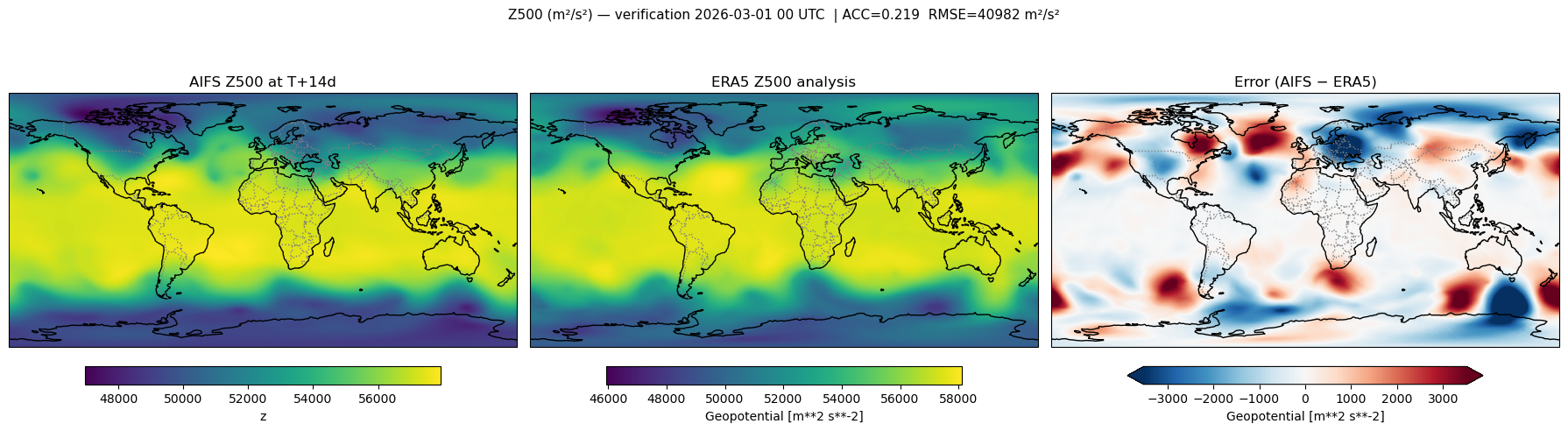
Evaluates the forecast with the Anomaly Correlation Coefficient (ACC) for Z500 at +14 days (2026-03-01 00 UTC) against the ERA5 analysis.
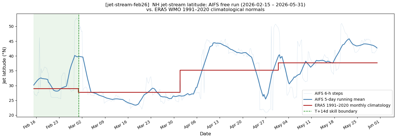
Diagnoses the Northern-Hemisphere jet-stream latitude from the AIFS 300 hPa zonal wind over the whole free-run period and compares it with the ERA5 WMO 1991–2020 climatological normals for the same calendar period.

Each experiment is isolated in its own icechunk branch of the outputs repository, named after the experiment variable set in the configuration cell below. Re-running with a different branch name (e.g. a different checkpoint or start date) keeps results completely independent.

[ ]:

import datetime as dt
import os
import tempfile
import time

import cartopy.crs as ccrs
import cartopy.feature as cfeature
import cdsapi
import icechunk
import matplotlib.dates as mdates
import matplotlib.pyplot as plt
import numpy as np
import pandas as pd
import xarray as xr

from aifs_modal import app, ingest, run_forecast

Configuration#

[ ]:

# --- experiment label (drives the icechunk branch for outputs) ---
experiment = "jet-stream-feb26"

# --- forecast window ---
start_date = dt.datetime(2026, 2, 15, 0, tzinfo=dt.UTC)
end_date = dt.datetime(2026, 5, 31, 0, tzinfo=dt.UTC)
lead_time = int((end_date - start_date).total_seconds() // 3600)  # hours
print(f"Experiment : {experiment}")
print(f"Start      : {start_date}")
print(f"End        : {end_date}")
print(f"Lead       : {lead_time} h  ({lead_time / 24:.0f} days)")

# --- skill-score reference ---
SKILL_LEAD_DAYS = 14
verification_date = start_date + dt.timedelta(days=SKILL_LEAD_DAYS)
print(f"Verification date (T+{SKILL_LEAD_DAYS}d): {verification_date}")

# --- storage ---
storage_bucket = "aifs-modal"
initial_conditions_prefix = "aifs-initial-conditions"
initial_conditions_branch = "main"
outputs_prefix = "aifs-outputs"
outputs_branch = experiment  # one branch per experiment

Experiment : jet-stream-feb26
Start      : 2026-02-15 00:00:00+00:00
End        : 2026-05-31 00:00:00+00:00
Lead       : 2520 h  (105 days)
Verification date (T+14d): 2026-03-01 00:00:00+00:00

1. Ingesting initial conditions#

AIFS needs two consecutive analysis states (t−6 h and t) as initial conditions.

[ ]:

initial_conditions_storage = icechunk.tigris_storage(
    bucket=storage_bucket,
    prefix=initial_conditions_prefix,
    region=os.getenv("AWS_REGION", None),
    access_key_id=os.environ["AWS_ACCESS_KEY_ID"],
    secret_access_key=os.environ["AWS_SECRET_ACCESS_KEY"],
)
initial_conditions_repo = icechunk.Repository.open(initial_conditions_storage)

for date in [start_date, start_date - dt.timedelta(hours=6)]:
    ingest.ensure_date_ingested(date, initial_conditions_repo)

  2026-03-06T11:11:08.094571Z  WARN aws_runtime::env_config::normalize: profile [plugins] ignored; sections in the AWS config file (other than [default]) must have a prefix i.e. [profile my-profile]
    at /home/conda/feedstock_root/build_artifacts/icechunk_1771452354651/_build_env/.cargo/registry/src/index.crates.io-1949cf8c6b5b557f/aws-runtime-1.5.18/src/env_config/normalize.rs:121

Initial conditions missing for 2026-02-15T00:00:00+00:00 (group: 2026-02-15/00z); ingesting now

By downloading data from the ECMWF open data dataset, you agree to the terms: Attribution 4.0 International (CC BY 4.0). Please attribute ECMWF when downloading this data.

Ingested initial conditions for 2026-02-15T00:00:00+00:00
Initial conditions missing for 2026-02-14T18:00:00+00:00 (group: 2026-02-14/18z); ingesting now

Ingested initial conditions for 2026-02-14T18:00:00+00:00

3. Loading forecast outputs#

[ ]:

outputs_storage = icechunk.tigris_storage(
    bucket=storage_bucket,
    prefix=outputs_prefix,
    region=os.getenv("AWS_REGION", None),
    access_key_id=os.environ["AWS_ACCESS_KEY_ID"],
    secret_access_key=os.environ["AWS_SECRET_ACCESS_KEY"],
)
outputs_repo = icechunk.Repository.open(outputs_storage)
outputs_session = outputs_repo.readonly_session(outputs_branch)

forecast_group = start_date.strftime("%Y-%m-%d/%Hz")
forecast_ds = xr.open_dataset(
    outputs_session.store,
    group=forecast_group,
    engine="zarr",
    zarr_format=3,
    chunks="auto",
)
forecast_ds

  2026-03-06T13:47:48.204011Z  WARN aws_runtime::env_config::normalize: profile [plugins] ignored; sections in the AWS config file (other than [default]) must have a prefix i.e. [profile my-profile]
    at /home/conda/feedstock_root/build_artifacts/icechunk_1771452354651/_build_env/.cargo/registry/src/index.crates.io-1949cf8c6b5b557f/aws-runtime-1.5.18/src/env_config/normalize.rs:121

<xarray.Dataset> Size: 178GB
Dimensions:     (valid_time: 420, lat: 721, lon: 1440, pressure: 13)
Coordinates:
  * valid_time  (valid_time) datetime64[ns] 3kB 2026-02-15T06:00:00 ... 2026-...
  * lat         (lat) float64 6kB 90.0 89.75 89.5 89.25 ... -89.5 -89.75 -90.0
  * lon         (lon) float64 12kB 0.0 0.25 0.5 0.75 ... 359.0 359.2 359.5 359.8
  * pressure    (pressure) int64 104B 50 100 150 200 250 ... 700 850 925 1000
Data variables: (12/30)
    100u        (valid_time, lat, lon) float32 2GB dask.array<chunksize=(32, 721, 1440), meta=np.ndarray>
    100v        (valid_time, lat, lon) float32 2GB dask.array<chunksize=(32, 721, 1440), meta=np.ndarray>
    10v         (valid_time, lat, lon) float32 2GB dask.array<chunksize=(32, 721, 1440), meta=np.ndarray>
    2t          (valid_time, lat, lon) float32 2GB dask.array<chunksize=(32, 721, 1440), meta=np.ndarray>
    hcc         (valid_time, lat, lon) float32 2GB dask.array<chunksize=(32, 721, 1440), meta=np.ndarray>
    lcc         (valid_time, lat, lon) float32 2GB dask.array<chunksize=(32, 721, 1440), meta=np.ndarray>
    ...          ...
    ro          (valid_time, lat, lon) float32 2GB dask.array<chunksize=(32, 721, 1440), meta=np.ndarray>
    u           (valid_time, pressure, lat, lon) float32 23GB dask.array<chunksize=(2, 13, 721, 1440), meta=np.ndarray>
    v           (valid_time, pressure, lat, lon) float32 23GB dask.array<chunksize=(2, 13, 721, 1440), meta=np.ndarray>
    z           (valid_time, pressure, lat, lon) float32 23GB dask.array<chunksize=(2, 13, 721, 1440), meta=np.ndarray>
    tcc         (valid_time, lat, lon) float32 2GB dask.array<chunksize=(32, 721, 1440), meta=np.ndarray>
    w           (valid_time, pressure, lat, lon) float32 23GB dask.array<chunksize=(2, 13, 721, 1440), meta=np.ndarray>

[ ]:

# quick sanity check: last valid time should be near end of May
print("First valid time:", forecast_ds.valid_time.values[0])
print("Last  valid time:", forecast_ds.valid_time.values[-1])
print("Number of time steps:", forecast_ds.dims["valid_time"])
print("Pressure levels:", forecast_ds.pressure.values)

First valid time: 2026-02-15T06:00:00.000000000
Last  valid time: 2026-05-31T00:00:00.000000000
Number of time steps: 420
Pressure levels: [  50  100  150  200  250  300  400  500  600  700  850  925 1000]

/tmp/ipykernel_2217402/1269242231.py:4: FutureWarning: The return type of `Dataset.dims` will be changed to return a set of dimension names in future, in order to be more consistent with `DataArray.dims`. To access a mapping from dimension names to lengths, please use `Dataset.sizes`.
  print("Number of time steps:", forecast_ds.dims["valid_time"])

5. Jet-stream latitude analysis#

The NH jet-stream latitude at each time step is defined as the latitude of the maximum zonal-mean 300 hPa zonal wind (U300) between 20°N and 80°N:

\[\phi_{\text{jet}}(t) = \arg\max_{\phi \in [20°N,\,80°N]} \overline{u}_{300}(\phi, t)\]

We compare the AIFS free-run jet latitude with the ERA5 1991–2020 monthly climatological jet latitude for the same calendar period.

5.1 AIFS jet-stream latitude time series#

[ ]:

# U300 from AIFS: dims (valid_time, pressure, lat, lon)
u300_aifs = forecast_ds["u"].sel(pressure=300, lat=slice(80, 20)).mean("lon").load()

# latitude of maximum zonal-mean U at each time step
jet_lat_aifs = u300_aifs.idxmax("lat").rename("jet_lat_aifs")

# also compute a 5-day (20-step) running mean for readability
jet_lat_aifs_rm = jet_lat_aifs.rolling(valid_time=20, center=True, min_periods=1).mean()

print("AIFS jet latitude — summary:")
print(f"  Mean : {float(jet_lat_aifs.mean()):.1f}°N")
print(f"  Std  : {float(jet_lat_aifs.std()):.1f}°")
print(f"  Min  : {float(jet_lat_aifs.min()):.1f}°N")
print(f"  Max  : {float(jet_lat_aifs.max()):.1f}°N")

AIFS jet latitude — summary:
  Mean : 34.0°N
  Std  : 8.6°
  Min  : 21.0°N
  Max  : 52.8°N

5.2 ERA5 1991–2020 climatological jet latitude#

We download ERA5 monthly mean U300 for February through May averaged over 1991–2020, then compute the monthly jet latitude.

[ ]:

def _era5_u300_monthly_clim(month, *, tmp_dir):
    """Download ERA5 monthly U300 mean for 1991–2020 and return the 30-yr mean."""
    out = os.path.join(tmp_dir, f"era5_u300_month{month:02d}_clim.nc")
    c.retrieve(
        "reanalysis-era5-pressure-levels-monthly-means",
        {
            "product_type": "monthly_averaged_reanalysis",
            "variable": "u_component_of_wind",
            "pressure_level": "300",
            "year": [str(y) for y in range(1991, 2021)],
            "month": f"{month:02d}",
            "time": "00:00",
            "grid": [0.25, 0.25],
            "area": [80, 0, 20, 360],  # NH jet region only
            "format": "netcdf",
        },
        out,
    )
    ds = xr.open_dataset(out)
    # variable name may be 'u' or 'u_component_of_wind' depending on CDS version
    u = ds[[v for v in ds if "u" in v.lower()][0]].squeeze()
    # 30-year mean, then zonal mean
    return u.mean("valid_time").mean("longitude")


# months covered by the free run: February (partial) through May
clim_months = [2, 3, 4, 5]
clim_jet_lats = {}

for m in clim_months:
    u300_clim = _era5_u300_monthly_clim(m, tmp_dir=era5_tmp)
    # latitude of max zonal-mean U300 (lat coord name from CDS is 'latitude')
    lat_dim = "latitude" if "latitude" in u300_clim.dims else "lat"
    clim_jet_lats[m] = float(u300_clim.idxmax(lat_dim))
    print(f"Month {m:2d}: climatological jet latitude = {clim_jet_lats[m]:.1f}°N")

2026-03-06 14:53:31,782 INFO Request ID is 6a386592-60ca-4d76-9572-375dcd6b0cb8
2026-03-06 14:53:31,841 INFO status has been updated to accepted
2026-03-06 14:59:50,891 INFO status has been updated to successful
2026-03-06 14:59:52,778 INFO Request ID is c05a6600-613c-4354-9cd6-b1c542db6055
2026-03-06 14:59:52,830 INFO status has been updated to accepted

Month  2: climatological jet latitude = 29.0°N

2026-03-06 15:00:06,261 INFO status has been updated to running
2026-03-06 15:00:25,338 INFO status has been updated to successful
2026-03-06 15:00:27,409 INFO Request ID is 66339a09-b7f3-4b0d-8569-75c7d6e6f81b

Month  3: climatological jet latitude = 27.8°N

2026-03-06 15:00:27,457 INFO status has been updated to accepted
2026-03-06 15:00:35,905 INFO status has been updated to running
2026-03-06 15:01:00,206 INFO status has been updated to successful
2026-03-06 15:01:01,976 INFO Request ID is 793d194d-32a3-4fa2-bb12-69f2cce1ad64

Month  4: climatological jet latitude = 35.2°N

2026-03-06 15:01:02,202 INFO status has been updated to accepted
2026-03-06 15:01:15,602 INFO status has been updated to running
2026-03-06 15:01:23,261 INFO status has been updated to successful

Month  5: climatological jet latitude = 37.8°N

5.3 Comparison: AIFS free-run vs. ERA5 1991–2020 climatology#

[ ]:

valid_times = jet_lat_aifs.valid_time.values  # numpy datetime64
times_pd = pd.DatetimeIndex(valid_times)

# map each valid time to the monthly climatological jet latitude
clim_ts = np.array([clim_jet_lats[ts.month] for ts in times_pd])

# --- plot ---
fig, ax = plt.subplots(figsize=(14, 5))

ax.plot(
    times_pd,
    jet_lat_aifs.values,
    color="steelblue",
    alpha=0.25,
    linewidth=0.6,
    label="AIFS 6-h steps",
)
ax.plot(
    times_pd,
    jet_lat_aifs_rm.values,
    color="steelblue",
    linewidth=2,
    label="AIFS 5-day running mean",
)
ax.step(
    times_pd,
    clim_ts,
    color="firebrick",
    linewidth=2,
    where="mid",
    label="ERA5 1991–2020 monthly climatology",
)

ax.axvspan(
    times_pd[0],
    pd.Timestamp(verification_date),
    alpha=0.08,
    color="green",
)
ax.axvline(
    pd.Timestamp(verification_date),
    color="green",
    linestyle="--",
    linewidth=1.2,
    label=f"T+{SKILL_LEAD_DAYS}d skill boundary",
)

ax.set_ylabel("Jet latitude (°N)", fontsize=12)
ax.set_xlabel("Date", fontsize=12)
ax.set_title(
    f"[{experiment}]  NH jet-stream latitude: AIFS free run "
    f"({start_date:%Y-%m-%d} – {end_date:%Y-%m-%d})\n"
    "vs. ERA5 WMO 1991–2020 climatological normals",
    fontsize=12,
)
ax.legend(fontsize=10)
ax.xaxis.set_major_formatter(mdates.DateFormatter("%b %d"))
ax.xaxis.set_major_locator(mdates.WeekdayLocator(byweekday=mdates.MO))
plt.xticks(rotation=30, ha="right")
plt.tight_layout()
plt.show()

/home/martibosch/data-science/aifs-modal-demo/.pixi/envs/default/lib/python3.12/site-packages/matplotlib/dates.py:449: UserWarning: no explicit representation of timezones available for np.datetime64
  d = d.astype('datetime64[us]')

../_images/user-guide_jet-stream-free-run_26_1.png

[ ]:

df = pd.DataFrame(
    {
        "valid_time": times_pd,
        "month": times_pd.month,
        "aifs_jet_lat": jet_lat_aifs.values,
        "era5_clim_lat": clim_ts,
    }
)
df["bias"] = df["aifs_jet_lat"] - df["era5_clim_lat"]

monthly_summary = (
    df.groupby("month")
    .agg(
        aifs_mean=("aifs_jet_lat", "mean"),
        aifs_std=("aifs_jet_lat", "std"),
        era5_clim=("era5_clim_lat", "first"),
        bias=("bias", "mean"),
    )
    .rename(index={2: "Feb", 3: "Mar", 4: "Apr", 5: "May"})
)

print(f"[{experiment}]  monthly jet-latitude summary")
print(monthly_summary.round(1).to_string())

[jet-stream-feb26]  monthly jet-latitude summary
       aifs_mean  aifs_std  era5_clim  bias
month
Feb         32.1       7.7       29.0   3.1
Mar         27.1       5.1       27.8  -0.6
Apr         36.4       9.1       35.2   1.2
May         39.3       6.1       37.8   1.6

AIFS Extended Free-Running Forecast: Mid-February to End of May 2026#

Configuration#

1. Ingesting initial conditions#

3. Loading forecast outputs#

4. Skill score at T+14 days#

4.1 ERA5 Z500 analysis for 2026-03-01#

4.2 ERA5 Z500 March climatology (1991–2020)#

4.3 Compute ACC and RMSE#

4.4 Spatial Z500 error map#

5. Jet-stream latitude analysis#

5.1 AIFS jet-stream latitude time series#

5.2 ERA5 1991–2020 climatological jet latitude#

5.3 Comparison: AIFS free-run vs. ERA5 1991–2020 climatology#

This Page

AIFS Extended Free-Running Forecast: Mid-February to End of May 2026#

Configuration#

1. Ingesting initial conditions#

2. Running the extended free-running forecast on Modal#

3. Loading forecast outputs#

4. Skill score at T+14 days#

4.1 ERA5 Z500 analysis for 2026-03-01#

4.2 ERA5 Z500 March climatology (1991–2020)#

4.3 Compute ACC and RMSE#

4.4 Spatial Z500 error map#

5. Jet-stream latitude analysis#

5.1 AIFS jet-stream latitude time series#

5.2 ERA5 1991–2020 climatological jet latitude#

5.3 Comparison: AIFS free-run vs. ERA5 1991–2020 climatology#

This Page