June 2025 European Heatwave Ensemble Reforecast

This notebook is an ensemble version of heatwave-reforecast.ipynb (deterministic). In order to compute the station-based ensemble Continuous Ranked Probability Score (CRPS), you need to the ensemble extra from the stationbench fork (e.g., pip install "stationbench[ensemble] @ git+https://github.com/martibosch/stationbench.git").

import datetime as dt
import os
import pathlib
import time

import cartopy.crs as ccrs
import cartopy.feature as cfeature
import icechunk
import matplotlib.pyplot as plt
import numpy as np
import pandas as pd
import seaborn as sns
import stationbench
import xarray as xr
from stationbench.utils import regions

from aifs_modal import app, ingest, run_ensemble_forecast

Set up

# experiment label
n_members = 10
experiment = "heatwave-2025-jun-ens"

# forecast window: init at heatwave onset for a clean 10-day medium/extended-range eval
start_date = dt.datetime(2025, 6, 20, 0, tzinfo=dt.UTC)
lead_time = 240  # in hours, i.e., until 2025-06-30 00 UTC
end_date = start_date + dt.timedelta(hours=lead_time)
print(f"Experiment : {experiment}")
print(f"Members    : {n_members}")
print(f"Start      : {start_date}")
print(f"End        : {end_date}  (T+{lead_time} h)")

# modal storage
storage_bucket = "aifs-modal"
initial_conditions_prefix = "aifs-initial-conditions"
initial_conditions_branch = "main"
outputs_prefix = "aifs-outputs-ens"
outputs_branch = experiment

# stationbench
region = "switzerland"
lat_slice = (44.5, 48.5)
lon_slice = (4.5, 11.5)
stationbench_dir = pathlib.Path("../data/stationbench")
stations_filepath = stationbench_dir / f"{experiment}-stations.nc"
era5_filepath = stationbench_dir / f"{experiment}-era5.nc"

# viz
figwidth = plt.rcParams["figure.figsize"][0]
figheight = plt.rcParams["figure.figsize"][1]

Experiment : heatwave-2025-jun-ens
Members    : 10
Start      : 2025-06-20 00:00:00+00:00
End        : 2025-06-30 00:00:00+00:00  (T+240 h)

1. Ingesting initial conditions

initial_conditions_storage = icechunk.tigris_storage(
    bucket=storage_bucket,
    prefix=initial_conditions_prefix,
    region=os.getenv("AWS_REGION", None),
    access_key_id=os.environ["AWS_ACCESS_KEY_ID"],
    secret_access_key=os.environ["AWS_SECRET_ACCESS_KEY"],
)
initial_conditions_repo = icechunk.Repository.open_or_create(initial_conditions_storage)

for date in [start_date - dt.timedelta(hours=6), start_date]:
    ingest.ensure_date_ingested(
        date, initial_conditions_repo, branch=initial_conditions_branch
    )

  2026-03-18T10:44:41.684971Z  WARN aws_runtime::env_config::normalize: profile [plugins] ignored; sections in the AWS config file (other than [default]) must have a prefix i.e. [profile my-profile]
    at /home/conda/feedstock_root/build_artifacts/icechunk_1773674412996/_build_env/.cargo/registry/src/index.crates.io-1949cf8c6b5b557f/aws-runtime-1.5.18/src/env_config/normalize.rs:121

Initial conditions already ingested for 2025-06-19T18:00:00+00:00 (group: 2025-06-19/18z); skipping
Initial conditions already ingested for 2025-06-20T00:00:00+00:00 (group: 2025-06-20/00z); skipping

2. Running the ensemble reforecast on Modal

All ensemble members run in parallel on separate GPUs using icechunk’s fork/merge pattern for distributed writes. The orchestrator function (run_ensemble_forecast) spawns one GPU container per member, merges the results, and commits:

{note} See the [How it works](../how-it-works.md) page for architecture diagrams showing how the parallel ensemble pipeline distributes work across GPUs and uses icechunk's fork/merge pattern for concurrent writes.

# with modal.enable_output():  # uncomment for live logs
with app.run():
    _start = time.perf_counter()
    run_ensemble_forecast.remote(
        start_date,
        storage_bucket,
        n_members=n_members,
        lead_time=lead_time,
        initial_conditions_prefix=initial_conditions_prefix,
        initial_conditions_branch=initial_conditions_branch,
        outputs_prefix=outputs_prefix,
        outputs_branch=outputs_branch,
        include_pressure_levels=False,
    )
    print(
        f"Ran {lead_time}-hour ensemble forecast with {n_members} members in "
        f"{time.perf_counter() - _start:.1f}s"
    )

Ran 240-hour ensemble forecast with 10 members in 477.9s

3. Loading ensemble forecast outputs

All members are stored in a single zarr group with an ensemble_member dimension:

# open outputs session
outputs_storage = icechunk.tigris_storage(
    bucket=storage_bucket,
    prefix=outputs_prefix,
    region=os.getenv("AWS_REGION", None),
    access_key_id=os.environ["AWS_ACCESS_KEY_ID"],
    secret_access_key=os.environ["AWS_SECRET_ACCESS_KEY"],
)
outputs_repo = icechunk.Repository.open_or_create(outputs_storage)
outputs_session = outputs_repo.readonly_session(outputs_branch)

# get forecasts
forecast_group = start_date.strftime("%Y-%m-%d/%Hz")
forecast_ds = xr.open_dataset(
    outputs_session.store,
    group=forecast_group,
    engine="zarr",
    zarr_format=3,
    chunks="auto",
)
print(
    f"{forecast_ds.sizes['ensemble_member']} members, "
    f"{forecast_ds.sizes['valid_time']} time steps"
)
forecast_ds

  2026-03-18T10:44:43.908107Z  WARN aws_runtime::env_config::normalize: profile [plugins] ignored; sections in the AWS config file (other than [default]) must have a prefix i.e. [profile my-profile]
    at /home/conda/feedstock_root/build_artifacts/icechunk_1773674412996/_build_env/.cargo/registry/src/index.crates.io-1949cf8c6b5b557f/aws-runtime-1.5.18/src/env_config/normalize.rs:121

10 members, 40 time steps

<xarray.Dataset> Size: 37GB
Dimensions:          (ensemble_member: 10, valid_time: 40, lat: 721, lon: 1440,
                      pressure: 13)
Coordinates:
  * ensemble_member  (ensemble_member) int64 80B 0 1 2 3 4 5 6 7 8 9
  * valid_time       (valid_time) datetime64[ns] 320B 2025-06-20T06:00:00 ......
  * lat              (lat) float64 6kB 90.0 89.75 89.5 ... -89.5 -89.75 -90.0
  * lon              (lon) float64 12kB 0.0 0.25 0.5 0.75 ... 359.2 359.5 359.8
  * pressure         (pressure) int64 104B 50 100 150 200 ... 700 850 925 1000
Data variables: (12/22)
    100u             (ensemble_member, valid_time, lat, lon) float32 2GB dask.array<chunksize=(5, 5, 721, 1440), meta=np.ndarray>
    100v             (ensemble_member, valid_time, lat, lon) float32 2GB dask.array<chunksize=(5, 5, 721, 1440), meta=np.ndarray>
    10v              (ensemble_member, valid_time, lat, lon) float32 2GB dask.array<chunksize=(5, 5, 721, 1440), meta=np.ndarray>
    hcc              (ensemble_member, valid_time, lat, lon) float32 2GB dask.array<chunksize=(5, 5, 721, 1440), meta=np.ndarray>
    10u              (ensemble_member, valid_time, lat, lon) float32 2GB dask.array<chunksize=(5, 5, 721, 1440), meta=np.ndarray>
    cp               (ensemble_member, valid_time, lat, lon) float32 2GB dask.array<chunksize=(5, 5, 721, 1440), meta=np.ndarray>
    ...               ...
    mcc              (ensemble_member, valid_time, lat, lon) float32 2GB dask.array<chunksize=(5, 5, 721, 1440), meta=np.ndarray>
    sp               (ensemble_member, valid_time, lat, lon) float32 2GB dask.array<chunksize=(5, 5, 721, 1440), meta=np.ndarray>
    tcw              (ensemble_member, valid_time, lat, lon) float32 2GB dask.array<chunksize=(5, 5, 721, 1440), meta=np.ndarray>
    strd             (ensemble_member, valid_time, lat, lon) float32 2GB dask.array<chunksize=(5, 5, 721, 1440), meta=np.ndarray>
    tp               (ensemble_member, valid_time, lat, lon) float32 2GB dask.array<chunksize=(5, 5, 721, 1440), meta=np.ndarray>
    tcc              (ensemble_member, valid_time, lat, lon) float32 2GB dask.array<chunksize=(5, 5, 721, 1440), meta=np.ndarray>

xarray.Dataset

• Dimensions:
  • ensemble_member: 10
  • valid_time: 40
  • lat: 721
  • lon: 1440
  • pressure: 13
• Coordinates: (5)
  • ensemble_member
    (ensemble_member)
    int64
    0 1 2 3 4 5 6 7 8 9

    array([0, 1, 2, 3, 4, 5, 6, 7, 8, 9])

  • valid_time
    (valid_time)
    datetime64[ns]
    2025-06-20T06:00:00 ... 2025-06-30

    axis :

    T

    standard_name :

    time

    array(['2025-06-20T06:00:00.000000000', '2025-06-20T12:00:00.000000000',
           '2025-06-20T18:00:00.000000000', '2025-06-21T00:00:00.000000000',
           '2025-06-21T06:00:00.000000000', '2025-06-21T12:00:00.000000000',
           '2025-06-21T18:00:00.000000000', '2025-06-22T00:00:00.000000000',
           '2025-06-22T06:00:00.000000000', '2025-06-22T12:00:00.000000000',
           '2025-06-22T18:00:00.000000000', '2025-06-23T00:00:00.000000000',
           '2025-06-23T06:00:00.000000000', '2025-06-23T12:00:00.000000000',
           '2025-06-23T18:00:00.000000000', '2025-06-24T00:00:00.000000000',
           '2025-06-24T06:00:00.000000000', '2025-06-24T12:00:00.000000000',
           '2025-06-24T18:00:00.000000000', '2025-06-25T00:00:00.000000000',
           '2025-06-25T06:00:00.000000000', '2025-06-25T12:00:00.000000000',
           '2025-06-25T18:00:00.000000000', '2025-06-26T00:00:00.000000000',
           '2025-06-26T06:00:00.000000000', '2025-06-26T12:00:00.000000000',
           '2025-06-26T18:00:00.000000000', '2025-06-27T00:00:00.000000000',
           '2025-06-27T06:00:00.000000000', '2025-06-27T12:00:00.000000000',
           '2025-06-27T18:00:00.000000000', '2025-06-28T00:00:00.000000000',
           '2025-06-28T06:00:00.000000000', '2025-06-28T12:00:00.000000000',
           '2025-06-28T18:00:00.000000000', '2025-06-29T00:00:00.000000000',
           '2025-06-29T06:00:00.000000000', '2025-06-29T12:00:00.000000000',
           '2025-06-29T18:00:00.000000000', '2025-06-30T00:00:00.000000000'],
          dtype='datetime64[ns]')

  • lat
    (lat)
    float64
    90.0 89.75 89.5 ... -89.75 -90.0

    standard_name :

    latitude

    axis :

    Y

    array([ 90.  ,  89.75,  89.5 , ..., -89.5 , -89.75, -90.  ], shape=(721,))

  • lon
    (lon)
    float64
    0.0 0.25 0.5 ... 359.2 359.5 359.8

    standard_name :

    longitude

    axis :

    X

    array([0.0000e+00, 2.5000e-01, 5.0000e-01, ..., 3.5925e+02, 3.5950e+02,
           3.5975e+02], shape=(1440,))

  • pressure
    (pressure)
    int64
    50 100 150 200 ... 700 850 925 1000

    array([  50,  100,  150,  200,  250,  300,  400,  500,  600,  700,  850,  925,
           1000])

• Data variables: (22)
  • 100u
    (ensemble_member, valid_time, lat, lon)
    float32
    dask.array<chunksize=(5, 5, 721, 1440), meta=np.ndarray>

    Array Chunk Bytes 1.55 GiB 99.01 MiB Shape (10, 40, 721, 1440) (5, 5, 721, 1440) Dask graph 16 chunks in 2 graph layers Data type float32 numpy.ndarray

  • 100v
    (ensemble_member, valid_time, lat, lon)
    float32
    dask.array<chunksize=(5, 5, 721, 1440), meta=np.ndarray>

    Array Chunk Bytes 1.55 GiB 99.01 MiB Shape (10, 40, 721, 1440) (5, 5, 721, 1440) Dask graph 16 chunks in 2 graph layers Data type float32 numpy.ndarray

  • 10v
    (ensemble_member, valid_time, lat, lon)
    float32
    dask.array<chunksize=(5, 5, 721, 1440), meta=np.ndarray>

    Array Chunk Bytes 1.55 GiB 99.01 MiB Shape (10, 40, 721, 1440) (5, 5, 721, 1440) Dask graph 16 chunks in 2 graph layers Data type float32 numpy.ndarray

  • hcc
    (ensemble_member, valid_time, lat, lon)
    float32
    dask.array<chunksize=(5, 5, 721, 1440), meta=np.ndarray>

    Array Chunk Bytes 1.55 GiB 99.01 MiB Shape (10, 40, 721, 1440) (5, 5, 721, 1440) Dask graph 16 chunks in 2 graph layers Data type float32 numpy.ndarray

  • 10u
    (ensemble_member, valid_time, lat, lon)
    float32
    dask.array<chunksize=(5, 5, 721, 1440), meta=np.ndarray>

    Array Chunk Bytes 1.55 GiB 99.01 MiB Shape (10, 40, 721, 1440) (5, 5, 721, 1440) Dask graph 16 chunks in 2 graph layers Data type float32 numpy.ndarray

  • cp
    (ensemble_member, valid_time, lat, lon)
    float32
    dask.array<chunksize=(5, 5, 721, 1440), meta=np.ndarray>

    Array Chunk Bytes 1.55 GiB 99.01 MiB Shape (10, 40, 721, 1440) (5, 5, 721, 1440) Dask graph 16 chunks in 2 graph layers Data type float32 numpy.ndarray

  • 2d
    (ensemble_member, valid_time, lat, lon)
    float32
    dask.array<chunksize=(5, 5, 721, 1440), meta=np.ndarray>

    Array Chunk Bytes 1.55 GiB 99.01 MiB Shape (10, 40, 721, 1440) (5, 5, 721, 1440) Dask graph 16 chunks in 2 graph layers Data type float32 numpy.ndarray

  • 2t
    (ensemble_member, valid_time, lat, lon)
    float32
    dask.array<chunksize=(5, 5, 721, 1440), meta=np.ndarray>

    Array Chunk Bytes 1.55 GiB 99.01 MiB Shape (10, 40, 721, 1440) (5, 5, 721, 1440) Dask graph 16 chunks in 2 graph layers Data type float32 numpy.ndarray

  • lcc
    (ensemble_member, valid_time, lat, lon)
    float32
    dask.array<chunksize=(5, 5, 721, 1440), meta=np.ndarray>

    Array Chunk Bytes 1.55 GiB 99.01 MiB Shape (10, 40, 721, 1440) (5, 5, 721, 1440) Dask graph 16 chunks in 2 graph layers Data type float32 numpy.ndarray

  • msl
    (ensemble_member, valid_time, lat, lon)
    float32
    dask.array<chunksize=(5, 5, 721, 1440), meta=np.ndarray>

    Array Chunk Bytes 1.55 GiB 99.01 MiB Shape (10, 40, 721, 1440) (5, 5, 721, 1440) Dask graph 16 chunks in 2 graph layers Data type float32 numpy.ndarray

  • ro
    (ensemble_member, valid_time, lat, lon)
    float32
    dask.array<chunksize=(5, 5, 721, 1440), meta=np.ndarray>

    Array Chunk Bytes 1.55 GiB 99.01 MiB Shape (10, 40, 721, 1440) (5, 5, 721, 1440) Dask graph 16 chunks in 2 graph layers Data type float32 numpy.ndarray

  • skt
    (ensemble_member, valid_time, lat, lon)
    float32
    dask.array<chunksize=(5, 5, 721, 1440), meta=np.ndarray>

    Array Chunk Bytes 1.55 GiB 99.01 MiB Shape (10, 40, 721, 1440) (5, 5, 721, 1440) Dask graph 16 chunks in 2 graph layers Data type float32 numpy.ndarray

  • ssrd
    (ensemble_member, valid_time, lat, lon)
    float32
    dask.array<chunksize=(5, 5, 721, 1440), meta=np.ndarray>

    Array Chunk Bytes 1.55 GiB 99.01 MiB Shape (10, 40, 721, 1440) (5, 5, 721, 1440) Dask graph 16 chunks in 2 graph layers Data type float32 numpy.ndarray

  • stl1
    (ensemble_member, valid_time, lat, lon)
    float32
    dask.array<chunksize=(5, 5, 721, 1440), meta=np.ndarray>

    Array Chunk Bytes 1.55 GiB 99.01 MiB Shape (10, 40, 721, 1440) (5, 5, 721, 1440) Dask graph 16 chunks in 2 graph layers Data type float32 numpy.ndarray

  • stl2
    (ensemble_member, valid_time, lat, lon)
    float32
    dask.array<chunksize=(5, 5, 721, 1440), meta=np.ndarray>

    Array Chunk Bytes 1.55 GiB 99.01 MiB Shape (10, 40, 721, 1440) (5, 5, 721, 1440) Dask graph 16 chunks in 2 graph layers Data type float32 numpy.ndarray

  • sf
    (ensemble_member, valid_time, lat, lon)
    float32
    dask.array<chunksize=(5, 5, 721, 1440), meta=np.ndarray>

    Array Chunk Bytes 1.55 GiB 99.01 MiB Shape (10, 40, 721, 1440) (5, 5, 721, 1440) Dask graph 16 chunks in 2 graph layers Data type float32 numpy.ndarray

  • mcc
    (ensemble_member, valid_time, lat, lon)
    float32
    dask.array<chunksize=(5, 5, 721, 1440), meta=np.ndarray>

    Array Chunk Bytes 1.55 GiB 99.01 MiB Shape (10, 40, 721, 1440) (5, 5, 721, 1440) Dask graph 16 chunks in 2 graph layers Data type float32 numpy.ndarray

  • sp
    (ensemble_member, valid_time, lat, lon)
    float32
    dask.array<chunksize=(5, 5, 721, 1440), meta=np.ndarray>

    Array Chunk Bytes 1.55 GiB 99.01 MiB Shape (10, 40, 721, 1440) (5, 5, 721, 1440) Dask graph 16 chunks in 2 graph layers Data type float32 numpy.ndarray

  • tcw
    (ensemble_member, valid_time, lat, lon)
    float32
    dask.array<chunksize=(5, 5, 721, 1440), meta=np.ndarray>

    Array Chunk Bytes 1.55 GiB 99.01 MiB Shape (10, 40, 721, 1440) (5, 5, 721, 1440) Dask graph 16 chunks in 2 graph layers Data type float32 numpy.ndarray

  • strd
    (ensemble_member, valid_time, lat, lon)
    float32
    dask.array<chunksize=(5, 5, 721, 1440), meta=np.ndarray>

    Array Chunk Bytes 1.55 GiB 99.01 MiB Shape (10, 40, 721, 1440) (5, 5, 721, 1440) Dask graph 16 chunks in 2 graph layers Data type float32 numpy.ndarray

  • tp
    (ensemble_member, valid_time, lat, lon)
    float32
    dask.array<chunksize=(5, 5, 721, 1440), meta=np.ndarray>

    Array Chunk Bytes 1.55 GiB 99.01 MiB Shape (10, 40, 721, 1440) (5, 5, 721, 1440) Dask graph 16 chunks in 2 graph layers Data type float32 numpy.ndarray

  • tcc
    (ensemble_member, valid_time, lat, lon)
    float32
    dask.array<chunksize=(5, 5, 721, 1440), meta=np.ndarray>

    Array Chunk Bytes 1.55 GiB 99.01 MiB Shape (10, 40, 721, 1440) (5, 5, 721, 1440) Dask graph 16 chunks in 2 graph layers Data type float32 numpy.ndarray

4. Prepare AIFS ensemble dataset for stationbench

The stationbench library expects a dataset with dimensions (time, prediction_timedelta, latitude, longitude) and, for ensemble metrics like CRPS, a member dimension. We rename ensemble_member to member to match stationbench conventions:

# get surface data
aifs_ds = forecast_ds.sel(pressure=1000).drop_vars("pressure")
# compute 10 m wind speed scalar
aifs_ds = aifs_ds.assign(**{"10si": np.sqrt(aifs_ds["10u"] ** 2 + aifs_ds["10v"] ** 2)})
# keep only stationbench variables
aifs_ds = aifs_ds[["2t", "10si"]]
# rename dims for stationbench: lat/lon and ensemble_member → member
aifs_ds = aifs_ds.rename(
    {"lat": "latitude", "lon": "longitude", "ensemble_member": "member"}
)
# replace valid_time with prediction_timedelta
init_time = np.datetime64(start_date.replace(tzinfo=None), "ns")
aifs_ds = aifs_ds.assign_coords(
    prediction_timedelta=forecast_ds.valid_time.values - init_time
).expand_dims({"time": [init_time]})
aifs_ds

<xarray.Dataset> Size: 3GB
Dimensions:               (time: 1, member: 10, valid_time: 40, latitude: 721,
                           longitude: 1440, prediction_timedelta: 40)
Coordinates:
  * time                  (time) datetime64[ns] 8B 2025-06-20
  * member                (member) int64 80B 0 1 2 3 4 5 6 7 8 9
  * valid_time            (valid_time) datetime64[ns] 320B 2025-06-20T06:00:0...
  * latitude              (latitude) float64 6kB 90.0 89.75 ... -89.75 -90.0
  * longitude             (longitude) float64 12kB 0.0 0.25 0.5 ... 359.5 359.8
  * prediction_timedelta  (prediction_timedelta) timedelta64[ns] 320B 06:00:0...
Data variables:
    2t                    (time, member, valid_time, latitude, longitude) float32 2GB dask.array<chunksize=(1, 5, 5, 721, 1440), meta=np.ndarray>
    10si                  (time, member, valid_time, latitude, longitude) float32 2GB dask.array<chunksize=(1, 5, 5, 721, 1440), meta=np.ndarray>

xarray.Dataset

• Dimensions:
  • time: 1
  • member: 10
  • valid_time: 40
  • latitude: 721
  • longitude: 1440
  • prediction_timedelta: 40
• Coordinates: (6)
  • time
    (time)
    datetime64[ns]
    2025-06-20

    array(['2025-06-20T00:00:00.000000000'], dtype='datetime64[ns]')

  • member
    (member)
    int64
    0 1 2 3 4 5 6 7 8 9

    array([0, 1, 2, 3, 4, 5, 6, 7, 8, 9])

  • valid_time
    (valid_time)
    datetime64[ns]
    2025-06-20T06:00:00 ... 2025-06-30

    axis :

    T

    standard_name :

    time

    array(['2025-06-20T06:00:00.000000000', '2025-06-20T12:00:00.000000000',
           '2025-06-20T18:00:00.000000000', '2025-06-21T00:00:00.000000000',
           '2025-06-21T06:00:00.000000000', '2025-06-21T12:00:00.000000000',
           '2025-06-21T18:00:00.000000000', '2025-06-22T00:00:00.000000000',
           '2025-06-22T06:00:00.000000000', '2025-06-22T12:00:00.000000000',
           '2025-06-22T18:00:00.000000000', '2025-06-23T00:00:00.000000000',
           '2025-06-23T06:00:00.000000000', '2025-06-23T12:00:00.000000000',
           '2025-06-23T18:00:00.000000000', '2025-06-24T00:00:00.000000000',
           '2025-06-24T06:00:00.000000000', '2025-06-24T12:00:00.000000000',
           '2025-06-24T18:00:00.000000000', '2025-06-25T00:00:00.000000000',
           '2025-06-25T06:00:00.000000000', '2025-06-25T12:00:00.000000000',
           '2025-06-25T18:00:00.000000000', '2025-06-26T00:00:00.000000000',
           '2025-06-26T06:00:00.000000000', '2025-06-26T12:00:00.000000000',
           '2025-06-26T18:00:00.000000000', '2025-06-27T00:00:00.000000000',
           '2025-06-27T06:00:00.000000000', '2025-06-27T12:00:00.000000000',
           '2025-06-27T18:00:00.000000000', '2025-06-28T00:00:00.000000000',
           '2025-06-28T06:00:00.000000000', '2025-06-28T12:00:00.000000000',
           '2025-06-28T18:00:00.000000000', '2025-06-29T00:00:00.000000000',
           '2025-06-29T06:00:00.000000000', '2025-06-29T12:00:00.000000000',
           '2025-06-29T18:00:00.000000000', '2025-06-30T00:00:00.000000000'],
          dtype='datetime64[ns]')

  • latitude
    (latitude)
    float64
    90.0 89.75 89.5 ... -89.75 -90.0

    standard_name :

    latitude

    axis :

    Y

    array([ 90.  ,  89.75,  89.5 , ..., -89.5 , -89.75, -90.  ], shape=(721,))

  • longitude
    (longitude)
    float64
    0.0 0.25 0.5 ... 359.2 359.5 359.8

    standard_name :

    longitude

    axis :

    X

    array([0.0000e+00, 2.5000e-01, 5.0000e-01, ..., 3.5925e+02, 3.5950e+02,
           3.5975e+02], shape=(1440,))

  • prediction_timedelta
    (prediction_timedelta)
    timedelta64[ns]
    0 days 06:00:00 ... 10 days 00:0...

    array([ 21600000000000,  43200000000000,  64800000000000,  86400000000000,
           108000000000000, 129600000000000, 151200000000000, 172800000000000,
           194400000000000, 216000000000000, 237600000000000, 259200000000000,
           280800000000000, 302400000000000, 324000000000000, 345600000000000,
           367200000000000, 388800000000000, 410400000000000, 432000000000000,
           453600000000000, 475200000000000, 496800000000000, 518400000000000,
           540000000000000, 561600000000000, 583200000000000, 604800000000000,
           626400000000000, 648000000000000, 669600000000000, 691200000000000,
           712800000000000, 734400000000000, 756000000000000, 777600000000000,
           799200000000000, 820800000000000, 842400000000000, 864000000000000],
          dtype='timedelta64[ns]')

• Data variables: (2)
  • 2t
    (time, member, valid_time, latitude, longitude)
    float32
    dask.array<chunksize=(1, 5, 5, 721, 1440), meta=np.ndarray>

    Array Chunk Bytes 1.55 GiB 99.01 MiB Shape (1, 10, 40, 721, 1440) (1, 5, 5, 721, 1440) Dask graph 16 chunks in 3 graph layers Data type float32 numpy.ndarray

  • 10si
    (time, member, valid_time, latitude, longitude)
    float32
    dask.array<chunksize=(1, 5, 5, 721, 1440), meta=np.ndarray>

    Array Chunk Bytes 1.55 GiB 99.01 MiB Shape (1, 10, 40, 721, 1440) (1, 5, 5, 721, 1440) Dask graph 16 chunks in 9 graph layers Data type float32 numpy.ndarray

5. Fetching MeteoSwiss station data

In order to benchmark the AIFS forecast with station measurements, we use meteora to download hourly temperature and wind-speed observations from MeteoSwiss automatic stations and convert the data into the stationbench input format (skipped automatically if already done):

ts_ds = xr.open_dataset(stations_filepath)
ts_ds

<xarray.Dataset> Size: 4MB
Dimensions:         (time: 1441, station_id: 157)
Coordinates:
  * time            (time) datetime64[ns] 12kB 2025-06-20 ... 2025-06-30
  * station_id      (station_id) <U3 2kB 'ABO' 'AEG' 'AIG' ... 'WFJ' 'WYN' 'ZER'
    longitude       (station_id) float64 1kB ...
    latitude        (station_id) float64 1kB ...
Data variables:
    2m_temperature  (time, station_id) float64 2MB ...
    10m_wind_speed  (time, station_id) float64 2MB ...

xarray.Dataset

• Dimensions:
  • time: 1441
  • station_id: 157
• Coordinates: (4)
  • time
    (time)
    datetime64[ns]
    2025-06-20 ... 2025-06-30

    array(['2025-06-20T00:00:00.000000000', '2025-06-20T00:10:00.000000000',
           '2025-06-20T00:20:00.000000000', ..., '2025-06-29T23:40:00.000000000',
           '2025-06-29T23:50:00.000000000', '2025-06-30T00:00:00.000000000'],
          shape=(1441,), dtype='datetime64[ns]')

  • station_id
    (station_id)
    <U3
    'ABO' 'AEG' 'AIG' ... 'WYN' 'ZER'

    array(['ABO', 'AEG', 'AIG', 'ALT', 'AND', 'ANT', 'ARH', 'ARO', 'ATT', 'BAN',
           'BAS', 'BEH', 'BER', 'BEZ', 'BIA', 'BIE', 'BIN', 'BIV', 'BIZ', 'BOL',
           'BOU', 'BRL', 'BRZ', 'BUF', 'BUS', 'CDF', 'CDM', 'CEV', 'CGI', 'CHA',
           'CHB', 'CHD', 'CHM', 'CHU', 'CHZ', 'CIM', 'CMA', 'COM', 'COV', 'COY',
           'CRM', 'DAV', 'DEM', 'DIA', 'DIS', 'DOL', 'EBK', 'EGH', 'EGO', 'EIN',
           'ELM', 'ENG', 'EVI', 'EVO', 'FAH', 'FLU', 'FRE', 'FRU', 'GEN', 'GES',
           'GIH', 'GLA', 'GOE', 'GOR', 'GOS', 'GRA', 'GRC', 'GRE', 'GRH', 'GRO',
           'GSB', 'GUE', 'GUT', 'GVE', 'HAI', 'HLL', 'HOE', 'ILZ', 'INT', 'JUN',
           'KLO', 'KOP', 'LAC', 'LAE', 'LAG', 'LAT', 'LEI', 'LUG', 'LUZ', 'MAG',
           'MAH', 'MAR', 'MAS', 'MER', 'MLS', 'MOA', 'MOB', 'MOE', 'MTE', 'MTR',
           'MUB', 'MVE', 'NAP', 'NAS', 'NEU', 'OBR', 'ORO', 'OTL', 'PAY', 'PFA',
           'PIL', 'PIO', 'PLF', 'PMA', 'PRE', 'PSI', 'PUY', 'QUI', 'RAG', 'REH',
           'ROB', 'ROE', 'RUE', 'SAE', 'SAG', 'SAM', 'SBE', 'SBO', 'SCM', 'SCU',
           'SHA', 'SIA', 'SIM', 'SIO', 'SMA', 'SMM', 'SPF', 'SRS', 'STC', 'STG',
           'STK', 'TAE', 'THU', 'TIT', 'UEB', 'ULR', 'VAB', 'VAD', 'VEV', 'VIO',
           'VIS', 'VIT', 'VLS', 'WAE', 'WFJ', 'WYN', 'ZER'], dtype='<U3')

  • longitude
    (station_id)
    float64
    ...

    [157 values with dtype=float64]

  • latitude
    (station_id)
    float64
    ...

    [157 values with dtype=float64]

• Data variables: (2)
  • 2m_temperature
    (time, station_id)
    float64
    ...

    [226237 values with dtype=float64]

  • 10m_wind_speed
    (time, station_id)
    float64
    ...

    [226237 values with dtype=float64]

6. Compute AIFS ensemble verification metrics

We now use stationbench.calculate_metrics, which interpolates the gridded AIFS forecast to the MeteoSwiss station locations and computes RMSE, MBE, and CRPS per station and per lead-time step for each variable. The CRPS metric evaluates the quality of the full ensemble distribution, not just the ensemble mean:

# add Switzerland region to stationbench if not already present
if region not in regions.region_dict:
    regions.add_region(region, lat_slice, lon_slice)
# compute stationbench metrics for AIFS forecast
metrics_ds = stationbench.calculate_metrics(
    forecast=aifs_ds,
    stations=ts_ds,
    start_date=start_date.strftime("%Y-%m-%d"),
    end_date=end_date.strftime("%Y-%m-%d"),
    region=region,
    name_2m_temperature="2t",
    name_10m_wind_speed="10si",
)
# exclude RMSE (maybe it would make sense to compute over the ensemble mean to compare
# with the deterministic case)
# TODO: stationbench-compatible approach to compute a subset of metrics only
metrics_ds = metrics_ds.sel(metric=["crps", "mbe"])
# show the dataset
metrics_ds

2026-03-18 12:00:47,461 - stationbench.calculate_metrics - INFO - Preparing stations data
2026-03-18 12:00:47,463 - stationbench.calculate_metrics - INFO - Selecting region: https://linestrings.com/bbox/#4.5,44.5,11.5,48.5
2026-03-18 12:00:47,476 - stationbench.calculate_metrics - INFO - Filtered stations: 157 -> 157
2026-03-18 12:00:47,515 - stationbench.calculate_metrics - INFO - Preparing forecast dataset
2026-03-18 12:00:47,530 - stationbench.calculate_metrics - INFO - Selecting region: https://linestrings.com/bbox/#4.5,44.5,11.5,48.5
2026-03-18 12:00:47,535 - stationbench.calculate_metrics - INFO - Converting longitudes from 0-360 to -180-180 range
2026-03-18 12:00:47,547 - stationbench.calculate_metrics - INFO - Renaming wind speed variable from 10si to 10m_wind_speed
2026-03-18 12:00:47,549 - stationbench.calculate_metrics - INFO - Renaming temperature variable from 2t to 2m_temperature
2026-03-18 12:00:47,551 - stationbench.calculate_metrics - INFO - Interpolating forecast to station locations
2026-03-18 12:01:39,767 - stationbench.calculate_metrics - INFO - Aligning stations with forecast valid times
2026-03-18 12:01:39,772 - stationbench.calculate_metrics - INFO - Calculating metrics
/home/martibosch/libraries/aifs-modal/.pixi/envs/user-guide/lib/python3.13/site-packages/stationbench/calculate_metrics.py:229: FutureWarning: In a future version of xarray the default value for join will change from join='outer' to join='exact'. This change will result in the following ValueError: cannot be aligned with join='exact' because index/labels/sizes are not equal along these coordinates (dimensions): 'metric' ('metric',) The recommendation is to set join explicitly for this case.
  return xr.merge(metrics_list)
/home/martibosch/libraries/aifs-modal/.pixi/envs/user-guide/lib/python3.13/site-packages/stationbench/calculate_metrics.py:229: FutureWarning: In a future version of xarray the default value for compat will change from compat='no_conflicts' to compat='override'. This is likely to lead to different results when combining overlapping variables with the same name. To opt in to new defaults and get rid of these warnings now use `set_options(use_new_combine_kwarg_defaults=True) or set compat explicitly.
  return xr.merge(metrics_list)
/home/martibosch/libraries/aifs-modal/.pixi/envs/user-guide/lib/python3.13/site-packages/stationbench/calculate_metrics.py:229: FutureWarning: In a future version of xarray the default value for compat will change from compat='no_conflicts' to compat='override'. This is likely to lead to different results when combining overlapping variables with the same name. To opt in to new defaults and get rid of these warnings now use `set_options(use_new_combine_kwarg_defaults=True) or set compat explicitly.
  return xr.merge(metrics_list)
/home/martibosch/libraries/aifs-modal/.pixi/envs/user-guide/lib/python3.13/site-packages/stationbench/calculate_metrics.py:229: FutureWarning: In a future version of xarray the default value for compat will change from compat='no_conflicts' to compat='override'. This is likely to lead to different results when combining overlapping variables with the same name. To opt in to new defaults and get rid of these warnings now use `set_options(use_new_combine_kwarg_defaults=True) or set compat explicitly.
  return xr.merge(metrics_list)
/home/martibosch/libraries/aifs-modal/.pixi/envs/user-guide/lib/python3.13/site-packages/stationbench/calculate_metrics.py:229: FutureWarning: In a future version of xarray the default value for compat will change from compat='no_conflicts' to compat='override'. This is likely to lead to different results when combining overlapping variables with the same name. To opt in to new defaults and get rid of these warnings now use `set_options(use_new_combine_kwarg_defaults=True) or set compat explicitly.
  return xr.merge(metrics_list)

<xarray.Dataset> Size: 80MB
Dimensions:         (member: 10, station_id: 157, lead_time: 40, metric: 2,
                     valid_time: 40)
Coordinates:
  * member          (member) int64 80B 0 1 2 3 4 5 6 7 8 9
  * station_id      (station_id) <U3 2kB 'ABO' 'AEG' 'AIG' ... 'WFJ' 'WYN' 'ZER'
    latitude        (station_id) float64 1kB 46.49 47.13 46.33 ... 47.26 46.03
    longitude       (station_id) float64 1kB 7.561 8.608 6.924 ... 7.787 7.752
  * lead_time       (lead_time) timedelta64[ns] 320B 0 days 06:00:00 ... 10 d...
  * metric          (metric) object 16B 'crps' 'mbe'
Dimensions without coordinates: valid_time
Data variables:
    2m_temperature  (metric, member, valid_time, station_id, lead_time) float64 40MB ...
    10m_wind_speed  (metric, member, valid_time, station_id, lead_time) float64 40MB ...

xarray.Dataset

• Dimensions:
  • member: 10
  • station_id: 157
  • lead_time: 40
  • metric: 2
  • valid_time: 40
• Coordinates: (6)
  • member
    (member)
    int64
    0 1 2 3 4 5 6 7 8 9

    array([0, 1, 2, 3, 4, 5, 6, 7, 8, 9])

  • station_id
    (station_id)
    <U3
    'ABO' 'AEG' 'AIG' ... 'WYN' 'ZER'

    array(['ABO', 'AEG', 'AIG', 'ALT', 'AND', 'ANT', 'ARH', 'ARO', 'ATT', 'BAN',
           'BAS', 'BEH', 'BER', 'BEZ', 'BIA', 'BIE', 'BIN', 'BIV', 'BIZ', 'BOL',
           'BOU', 'BRL', 'BRZ', 'BUF', 'BUS', 'CDF', 'CDM', 'CEV', 'CGI', 'CHA',
           'CHB', 'CHD', 'CHM', 'CHU', 'CHZ', 'CIM', 'CMA', 'COM', 'COV', 'COY',
           'CRM', 'DAV', 'DEM', 'DIA', 'DIS', 'DOL', 'EBK', 'EGH', 'EGO', 'EIN',
           'ELM', 'ENG', 'EVI', 'EVO', 'FAH', 'FLU', 'FRE', 'FRU', 'GEN', 'GES',
           'GIH', 'GLA', 'GOE', 'GOR', 'GOS', 'GRA', 'GRC', 'GRE', 'GRH', 'GRO',
           'GSB', 'GUE', 'GUT', 'GVE', 'HAI', 'HLL', 'HOE', 'ILZ', 'INT', 'JUN',
           'KLO', 'KOP', 'LAC', 'LAE', 'LAG', 'LAT', 'LEI', 'LUG', 'LUZ', 'MAG',
           'MAH', 'MAR', 'MAS', 'MER', 'MLS', 'MOA', 'MOB', 'MOE', 'MTE', 'MTR',
           'MUB', 'MVE', 'NAP', 'NAS', 'NEU', 'OBR', 'ORO', 'OTL', 'PAY', 'PFA',
           'PIL', 'PIO', 'PLF', 'PMA', 'PRE', 'PSI', 'PUY', 'QUI', 'RAG', 'REH',
           'ROB', 'ROE', 'RUE', 'SAE', 'SAG', 'SAM', 'SBE', 'SBO', 'SCM', 'SCU',
           'SHA', 'SIA', 'SIM', 'SIO', 'SMA', 'SMM', 'SPF', 'SRS', 'STC', 'STG',
           'STK', 'TAE', 'THU', 'TIT', 'UEB', 'ULR', 'VAB', 'VAD', 'VEV', 'VIO',
           'VIS', 'VIT', 'VLS', 'WAE', 'WFJ', 'WYN', 'ZER'], dtype='<U3')

  • latitude
    (station_id)
    float64
    46.49 47.13 46.33 ... 47.26 46.03

    array([46.491703, 47.133636, 46.326647, 46.887069, 46.610139, 46.630914,
           47.483631, 46.792661, 46.0991  , 46.977806, 47.541142, 46.409158,
           46.990744, 47.557256, 46.336053, 46.524908, 46.367661, 46.462494,
           47.508828, 46.623519, 46.393447, 46.983844, 46.740719, 46.648408,
           47.384381, 47.082947, 46.391525, 46.320486, 46.401053, 47.131761,
           46.67015 , 46.479819, 47.049169, 46.870572, 47.188278, 46.200467,
           46.842275, 46.459517, 46.418039, 47.180811, 47.047581, 46.812969,
           47.351706, 46.32675 , 46.706569, 46.424794, 47.273389, 46.426528,
           47.179428, 47.133042, 46.923742, 46.821639, 46.182953, 46.112211,
           47.423814, 46.889436, 46.840622, 46.599003, 45.927592, 46.996069,
           46.849447, 47.034586, 47.363147, 45.983644, 46.692678, 46.7714  ,
           46.195314, 47.179097, 46.571689, 46.255075, 45.869092, 46.652475,
           47.601733, 46.247519, 47.651242, 47.697278, 47.370864, 46.775039,
           46.672033, 46.547556, 47.479611, 47.11885 , 47.179197, 47.481933,
           46.939633, 46.627275, 47.597361, 46.004217, 47.036439, 46.160025,
           46.736978, 46.118903, 46.656486, 46.732222, 46.546197, 47.243847,
           46.071019, 47.572197, 46.147897, 46.410103, 46.973278, 46.298806,
           47.004667, 46.817164, 47.000067, 47.376608, 46.572269, 46.172256,
           46.811581, 47.376817, 46.978869, 46.514811, 46.747717, 46.577181,
           46.483683, 47.536475, 46.512283, 47.128739, 47.016631, 47.427694,
           46.347217, 46.443067, 47.434572, 47.249447, 47.081064, 46.526247,
           46.463542, 45.843444, 47.224933, 46.793275, 47.689842, 46.432331,
           46.196825, 46.21865 , 47.377925, 46.602256, 46.947042, 46.975506,
           47.571767, 47.425475, 47.668628, 47.479892, 46.749853, 46.770608,
           47.351364, 46.504881, 46.755039, 47.127472, 46.471239, 46.353019,
           46.3029  , 46.621778, 46.627758, 47.220958, 46.833325, 47.255025,
           46.029272])

  • longitude
    (station_id)
    float64
    7.561 8.608 6.924 ... 7.787 7.752

    array([ 7.560703,  8.608206,  6.924472,  8.621894,  9.431981,  8.580553,
            9.56685 ,  9.679014,  7.26865 ,  7.528667,  7.583525, 10.019567,
            7.464061,  8.233325,  8.978197,  6.342386,  8.192306,  9.668639,
            9.266797,  7.384206,  6.857006,  6.610297,  8.060864, 10.2672  ,
            8.07955 ,  6.792314,  7.098239,  8.603161,  6.227722,  7.054367,
            6.312428,  7.139656,  6.978825,  9.530761,  8.464642,  8.79165 ,
            9.180042,  8.935486,  9.821308,  7.090656,  7.059147,  9.843558,
            7.349567,  7.203781,  8.853478,  6.099453,  9.108494,  8.092728,
            8.004758,  8.756556,  9.175347,  8.410514,  7.026747,  7.508631,
            6.941194,  8.020336,  6.576369,  7.657542,  9.017875,  8.523442,
            8.190225,  9.066961,  7.973733,  7.785944,  8.595364,  7.113736,
            7.836822,  7.415144,  8.333256,  9.163758,  7.170683,  8.615531,
            9.279428,  6.127742,  9.023911,  8.470464,  8.941644,  9.215353,
            7.87045 ,  7.985444,  8.535961,  7.605503,  8.858686,  8.397222,
            7.806425,  9.753706,  8.1882  ,  8.960322,  8.301022,  8.933672,
            6.567983,  7.016597,  7.069669,  8.169247,  7.017753,  8.232831,
            7.225272,  7.877911,  7.624033,  8.924742,  7.278217,  7.460814,
            7.940117, 10.2614  ,  6.953297,  9.612706,  6.858239,  8.787494,
            6.942469,  8.754864,  8.252256,  8.688039,  7.266264,  9.529544,
            6.443   ,  8.226944,  6.667517,  9.21605 ,  9.502594,  8.517953,
           10.063031,  8.513389,  7.879414,  9.343469,  8.636967,  9.879469,
            9.1847  ,  8.932364,  8.9403  , 10.283267,  8.620142,  9.762325,
            8.056336,  7.330203,  8.565742, 10.426314,  8.012442,  9.668075,
            7.687094,  9.398528,  8.981433,  8.904928,  7.585222,  8.425981,
            8.490225,  8.308236,  9.554433,  9.517578,  6.815056,  9.6278  ,
            7.842958,  6.710069,  9.188711,  8.677706,  9.806394,  7.787475,
            7.752433])

  • lead_time
    (lead_time)
    timedelta64[ns]
    0 days 06:00:00 ... 10 days 00:0...

    array([ 21600000000000,  43200000000000,  64800000000000,  86400000000000,
           108000000000000, 129600000000000, 151200000000000, 172800000000000,
           194400000000000, 216000000000000, 237600000000000, 259200000000000,
           280800000000000, 302400000000000, 324000000000000, 345600000000000,
           367200000000000, 388800000000000, 410400000000000, 432000000000000,
           453600000000000, 475200000000000, 496800000000000, 518400000000000,
           540000000000000, 561600000000000, 583200000000000, 604800000000000,
           626400000000000, 648000000000000, 669600000000000, 691200000000000,
           712800000000000, 734400000000000, 756000000000000, 777600000000000,
           799200000000000, 820800000000000, 842400000000000, 864000000000000],
          dtype='timedelta64[ns]')

  • metric
    (metric)
    object
    'crps' 'mbe'

    array(['crps', 'mbe'], dtype=object)

• Data variables: (2)
  • 2m_temperature
    (metric, member, valid_time, station_id, lead_time)
    float64
    3.834 11.13 7.434 ... -11.98 -3.278

    array([[[[[  3.83380649,  11.13380649,   7.43380649, ...,
                13.03380649,  11.93380649,   6.73380649],
              [         nan,          nan,          nan, ...,
                        nan,          nan,          nan],
              [  2.94415506,  10.14415506,  10.44415506, ...,
                12.84415506,  13.04415506,   4.44415506],
              ...,
              [  1.32531307,   1.05464188,   1.22531307, ...,
                 4.05464188,   1.05464188,   0.20655988],
              [  1.67493897,   9.77493897,   8.47493897, ...,
                13.67493897,  12.27493897,   2.07493897],
              [  2.29067372,  15.49067372,   9.99067372, ...,
                16.19067372,  13.39067372,   4.69067372]],
    
             [[  4.03537532,   2.63145554,   0.546617  , ...,
                 4.53145554,   3.43145554,   1.13537532],
              [         nan,          nan,          nan, ...,
                        nan,          nan,          nan],
              [  4.13962369,   2.26420337,   2.56420337, ...,
                 4.96420337,   5.16420337,   2.63962369],
    ...
                 3.95321999,   6.95321999,   8.45321999],
              [  8.30831091,   0.20831091,   1.50831091, ...,
                -3.69168909,  -2.29168909,   7.90831091],
              [  5.13811684,  -8.06188316,  -2.56188316, ...,
                -8.76188316,  -5.96188316,   2.73811684]],
    
             [[ -2.9116809 , -10.2116809 ,  -6.5116809 , ...,
               -12.1116809 , -11.0116809 ,  -5.8116809 ],
              [         nan,          nan,          nan, ...,
                        nan,          nan,          nan],
              [ -1.87670905,  -9.07670905,  -9.37670905, ...,
               -11.77670905, -11.97670905,  -3.37670905],
              ...,
              [  3.72816865,   0.52816865,   3.62816865, ...,
                -2.47183135,   0.52816865,   2.02816865],
              [  1.6634151 ,  -6.4365849 ,  -5.1365849 , ...,
               -10.3365849 ,  -8.9365849 ,   1.2634151 ],
              [ -0.87813108, -14.07813108,  -8.57813108, ...,
               -14.77813108, -11.97813108,  -3.27813108]]]]],
          shape=(2, 10, 40, 157, 40))

  • 10m_wind_speed
    (metric, member, valid_time, station_id, lead_time)
    float64
    0.2893 4.289 ... 0.5525 -1.348

    array([[[[[ 2.89269680e-01,  4.28926968e+00,  6.89269680e-01, ...,
                2.48926968e+00,  1.92667770e-01,  2.22669250e-02],
              [ 2.01170115e-01,  2.40389664e+00,  1.10389664e+00, ...,
                2.40389664e+00,  1.10389664e+00,  8.03896635e-01],
              [ 5.91501582e-01,  2.96259652e+00,  9.62596520e-01, ...,
                2.86259652e+00,  7.62596520e-01,  2.28839627e-02],
              ...,
              [ 1.34536629e+00,  3.44536629e+00,  5.04536629e+00, ...,
                2.64536629e+00,  5.44536629e+00,  2.46308789e-01],
              [ 2.10323462e+00,  3.30323462e+00,  2.40323462e+00, ...,
                2.00323462e+00,  4.03234620e-01,  9.88139106e-01],
              [ 3.71863371e-02,  2.60239240e+00,  5.10239240e+00, ...,
                3.10239240e+00,  3.71863371e-02,  1.80239240e+00]],
    
             [[ 4.54881824e-01,  2.96521971e+00,  2.31698965e-01, ...,
                1.16521971e+00,  5.34881824e-01,  7.74881824e-01],
              [ 1.63936992e+00,  7.59315635e-01,  1.86299694e-01, ...,
                7.59315635e-01,  1.86299694e-01,  4.39369920e-01],
              [ 1.27613572e+00,  2.05387573e+00,  1.25534340e-01, ...,
                1.95387573e+00,  6.03528317e-02,  5.76135716e-01],
    ...
               -2.54805307e+00, -5.34805307e+00, -1.48053072e-01],
              [-2.29696741e+00, -3.49696741e+00, -2.59696741e+00, ...,
               -2.19696741e+00, -5.96967412e-01,  1.20303259e+00],
              [ 2.93940844e-01, -2.40605916e+00, -4.90605916e+00, ...,
               -2.90605916e+00,  2.93940844e-01, -1.60605916e+00]],
    
             [[ 1.54278008e-02, -3.98457220e+00, -3.84572199e-01, ...,
               -2.18457220e+00,  1.15427801e-01,  4.15427801e-01],
              [ 7.53771806e-01, -2.04622819e+00, -7.46228194e-01, ...,
               -2.04622819e+00, -7.46228194e-01, -4.46228194e-01],
              [ 9.01836008e-01, -2.79816399e+00, -7.98163992e-01, ...,
               -2.69816399e+00, -5.98163992e-01,  2.01836008e-01],
              ...,
              [-1.42641327e+00, -3.52641327e+00, -5.12641327e+00, ...,
               -2.72641327e+00, -5.52641327e+00, -3.26413275e-01],
              [-2.80137586e+00, -4.00137586e+00, -3.10137586e+00, ...,
               -2.70137586e+00, -1.10137586e+00,  6.98624144e-01],
              [ 5.52450172e-01, -2.14754983e+00, -4.64754983e+00, ...,
               -2.64754983e+00,  5.52450172e-01, -1.34754983e+00]]]]],
          shape=(2, 10, 40, 157, 40))

We can now compute the MBE, and CRPS averaged across all stations for the medium-range (days 1-7) and extended-range (days 7-10) bins:

bins = {
    "days 1-7": (np.timedelta64(1, "D"), np.timedelta64(7, "D")),
    "days 7-10": (np.timedelta64(7, "D"), np.timedelta64(10, "D")),
}

rows = []
for label, (t0, t1) in bins.items():
    row = {"bin": f"AIFS-ENS {label}"}
    for metric_name in metrics_ds.metric.values:
        val = (
            metrics_ds["2m_temperature"]
            .sel(metric=metric_name, lead_time=slice(t0, t1))
            .mean()
            .item()
        )
        col = f"{metric_name.upper()} (K)"
        row[col] = val
    rows.append(row)

pd.DataFrame(rows).set_index("bin")

	CRPS (K)	MBE (K)
bin
AIFS-ENS days 1-7	4.616505	-0.892011
AIFS-ENS days 7-10	4.943851	-1.861350

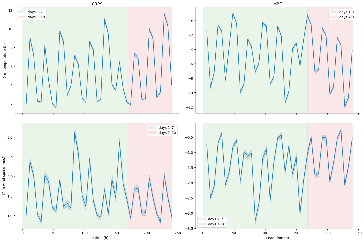
Station-mean metrics as a function of lead time, including CRPS:

for metric_name in metrics_ds.metric.values:
    df = metrics_ds.drop_vars(["latitude", "longitude"]).sel(
        metric=metric_name, drop=True
    )
    break
df

<xarray.Dataset> Size: 40MB
Dimensions:         (member: 10, station_id: 157, lead_time: 40, valid_time: 40)
Coordinates:
  * member          (member) int64 80B 0 1 2 3 4 5 6 7 8 9
  * station_id      (station_id) <U3 2kB 'ABO' 'AEG' 'AIG' ... 'WFJ' 'WYN' 'ZER'
  * lead_time       (lead_time) timedelta64[ns] 320B 0 days 06:00:00 ... 10 d...
Dimensions without coordinates: valid_time
Data variables:
    2m_temperature  (member, valid_time, station_id, lead_time) float64 20MB ...
    10m_wind_speed  (member, valid_time, station_id, lead_time) float64 20MB ...

xarray.Dataset

• Dimensions:
  • member: 10
  • station_id: 157
  • lead_time: 40
  • valid_time: 40
• Coordinates: (3)
  • member
    (member)
    int64
    0 1 2 3 4 5 6 7 8 9

    array([0, 1, 2, 3, 4, 5, 6, 7, 8, 9])

  • station_id
    (station_id)
    <U3
    'ABO' 'AEG' 'AIG' ... 'WYN' 'ZER'

    array(['ABO', 'AEG', 'AIG', 'ALT', 'AND', 'ANT', 'ARH', 'ARO', 'ATT', 'BAN',
           'BAS', 'BEH', 'BER', 'BEZ', 'BIA', 'BIE', 'BIN', 'BIV', 'BIZ', 'BOL',
           'BOU', 'BRL', 'BRZ', 'BUF', 'BUS', 'CDF', 'CDM', 'CEV', 'CGI', 'CHA',
           'CHB', 'CHD', 'CHM', 'CHU', 'CHZ', 'CIM', 'CMA', 'COM', 'COV', 'COY',
           'CRM', 'DAV', 'DEM', 'DIA', 'DIS', 'DOL', 'EBK', 'EGH', 'EGO', 'EIN',
           'ELM', 'ENG', 'EVI', 'EVO', 'FAH', 'FLU', 'FRE', 'FRU', 'GEN', 'GES',
           'GIH', 'GLA', 'GOE', 'GOR', 'GOS', 'GRA', 'GRC', 'GRE', 'GRH', 'GRO',
           'GSB', 'GUE', 'GUT', 'GVE', 'HAI', 'HLL', 'HOE', 'ILZ', 'INT', 'JUN',
           'KLO', 'KOP', 'LAC', 'LAE', 'LAG', 'LAT', 'LEI', 'LUG', 'LUZ', 'MAG',
           'MAH', 'MAR', 'MAS', 'MER', 'MLS', 'MOA', 'MOB', 'MOE', 'MTE', 'MTR',
           'MUB', 'MVE', 'NAP', 'NAS', 'NEU', 'OBR', 'ORO', 'OTL', 'PAY', 'PFA',
           'PIL', 'PIO', 'PLF', 'PMA', 'PRE', 'PSI', 'PUY', 'QUI', 'RAG', 'REH',
           'ROB', 'ROE', 'RUE', 'SAE', 'SAG', 'SAM', 'SBE', 'SBO', 'SCM', 'SCU',
           'SHA', 'SIA', 'SIM', 'SIO', 'SMA', 'SMM', 'SPF', 'SRS', 'STC', 'STG',
           'STK', 'TAE', 'THU', 'TIT', 'UEB', 'ULR', 'VAB', 'VAD', 'VEV', 'VIO',
           'VIS', 'VIT', 'VLS', 'WAE', 'WFJ', 'WYN', 'ZER'], dtype='<U3')

  • lead_time
    (lead_time)
    timedelta64[ns]
    0 days 06:00:00 ... 10 days 00:0...

    array([ 21600000000000,  43200000000000,  64800000000000,  86400000000000,
           108000000000000, 129600000000000, 151200000000000, 172800000000000,
           194400000000000, 216000000000000, 237600000000000, 259200000000000,
           280800000000000, 302400000000000, 324000000000000, 345600000000000,
           367200000000000, 388800000000000, 410400000000000, 432000000000000,
           453600000000000, 475200000000000, 496800000000000, 518400000000000,
           540000000000000, 561600000000000, 583200000000000, 604800000000000,
           626400000000000, 648000000000000, 669600000000000, 691200000000000,
           712800000000000, 734400000000000, 756000000000000, 777600000000000,
           799200000000000, 820800000000000, 842400000000000, 864000000000000],
          dtype='timedelta64[ns]')

• Data variables: (2)
  • 2m_temperature
    (member, valid_time, station_id, lead_time)
    float64
    3.834 11.13 7.434 ... 11.31 2.609

    array([[[[ 3.83380649, 11.13380649,  7.43380649, ..., 13.03380649,
              11.93380649,  6.73380649],
             [        nan,         nan,         nan, ...,         nan,
                      nan,         nan],
             [ 2.94415506, 10.14415506, 10.44415506, ..., 12.84415506,
              13.04415506,  4.44415506],
             ...,
             [ 1.32531307,  1.05464188,  1.22531307, ...,  4.05464188,
               1.05464188,  0.20655988],
             [ 1.67493897,  9.77493897,  8.47493897, ..., 13.67493897,
              12.27493897,  2.07493897],
             [ 2.29067372, 15.49067372,  9.99067372, ..., 16.19067372,
              13.39067372,  4.69067372]],
    
            [[ 4.03537532,  2.63145554,  0.546617  , ...,  4.53145554,
               3.43145554,  1.13537532],
             [        nan,         nan,         nan, ...,         nan,
                      nan,         nan],
             [ 4.13962369,  2.26420337,  2.56420337, ...,  4.96420337,
               5.16420337,  2.63962369],
    ...
             [ 8.1396868 ,  4.9396868 ,  8.0396868 , ...,  1.9396868 ,
               4.9396868 ,  6.4396868 ],
             [ 6.86385003,  0.23790597,  0.57917023, ...,  3.38056602,
               1.98056602,  6.46385003],
             [ 3.47479371,  8.12285672,  2.62285672, ...,  8.82285672,
               6.02285672,  1.13529392]],
    
            [[ 2.78044009, 10.08044009,  6.38044009, ..., 11.98044009,
              10.88044009,  5.68044009],
             [        nan,         nan,         nan, ...,         nan,
                      nan,         nan],
             [ 1.77195727,  8.97195727,  9.27195727, ..., 11.67195727,
              11.87195727,  3.27195727],
             ...,
             [ 2.37609985,  0.26595313,  2.27609985, ...,  2.82866467,
               0.26595313,  0.67609985],
             [ 0.32822329,  6.99545558,  5.69545558, ..., 10.89545558,
               9.49545558,  0.23054994],
             [ 0.34570876, 13.40905417,  7.90905417, ..., 14.10905417,
              11.30905417,  2.60905417]]]], shape=(10, 40, 157, 40))

  • 10m_wind_speed
    (member, valid_time, station_id, lead_time)
    float64
    0.2893 4.289 ... 0.08613 1.577

    array([[[[0.28926968, 4.28926968, 0.68926968, ..., 2.48926968,
              0.19266777, 0.02226693],
             [0.20117011, 2.40389664, 1.10389664, ..., 2.40389664,
              1.10389664, 0.80389664],
             [0.59150158, 2.96259652, 0.96259652, ..., 2.86259652,
              0.76259652, 0.02288396],
             ...,
             [1.34536629, 3.44536629, 5.04536629, ..., 2.64536629,
              5.44536629, 0.24630879],
             [2.10323462, 3.30323462, 2.40323462, ..., 2.00323462,
              0.40323462, 0.98813911],
             [0.03718634, 2.6023924 , 5.1023924 , ..., 3.1023924 ,
              0.03718634, 1.8023924 ]],
    
            [[0.45488182, 2.96521971, 0.23169896, ..., 1.16521971,
              0.53488182, 0.77488182],
             [1.63936992, 0.75931564, 0.18629969, ..., 0.75931564,
              0.18629969, 0.43936992],
             [1.27613572, 2.05387573, 0.12553434, ..., 1.95387573,
              0.06035283, 0.57613572],
    ...
             [0.68424139, 2.78424139, 4.38424139, ..., 1.98424139,
              4.78424139, 0.09239246],
             [1.26436521, 2.46436521, 1.56436521, ..., 1.16436521,
              0.12947247, 1.49743058],
             [0.13193089, 2.301373  , 4.801373  , ..., 2.801373  ,
              0.13193089, 1.501373  ]],
    
            [[0.06373162, 3.73249816, 0.23632742, ..., 1.93249816,
              0.06652211, 0.24509111],
             [0.1186687 , 2.25183102, 0.95183102, ..., 2.25183102,
              0.95183102, 0.65183102],
             [0.66458077, 2.61412601, 0.61412601, ..., 2.51412601,
              0.45309071, 0.06037751],
             ...,
             [1.22012013, 3.32012013, 4.92012013, ..., 2.52012013,
              5.32012013, 0.14948056],
             [2.1027774 , 3.3027774 , 2.4027774 , ..., 2.0027774 ,
              0.44761822, 0.77570838],
             [0.08613062, 2.3770638 , 4.8770638 , ..., 2.8770638 ,
              0.08613062, 1.5770638 ]]]], shape=(10, 40, 157, 40))

# plot args
aspect = 1.5
lead_time_label = "Lead time (h)"
medium_color = sns.color_palette()[2]
extended_color = sns.color_palette()[3]
alpha = 0.1

# get long metrics data frame for seaborn
# 1. drop longitude/latitude
# 2. reduce parallel valid_time/lead_time to lead_time only
# 3. convert to pandas data frame
plot_df = (
    metrics_ds.drop_vars(["latitude", "longitude"])
    # .sel(metric=metric, drop=True)
    .isel(valid_time=xr.DataArray(range(len(metrics_ds.valid_time)), dims="valid_time"))
    .isel(valid_time=0, drop=True)
    .to_dataframe()
    .reset_index()
)
# 4. convert lead time to hours (int) and rename it for a nicer label
plot_df[lead_time_label] = (plot_df["lead_time"] / np.timedelta64(1, "h")).astype(int)
plot_df = plot_df.drop(columns=["lead_time"])
# 5. stack variables
plot_df = plot_df.melt(
    id_vars=plot_df.columns.drop(metrics_ds.data_vars), value_vars=metrics_ds.data_vars
)
# 6. nicer labels
plot_df["metric"] = plot_df["metric"].str.upper()
plot_df["variable"] = plot_df["variable"].map(
    {"2m_temperature": "2 m temperature (K)", "10m_wind_speed": "10 m wind speed (m/s)"}
)
# seaborn plot
g = sns.relplot(
    data=plot_df,
    x=lead_time_label,
    y="value",
    row="variable",
    col="metric",
    kind="line",
    facet_kws=dict(sharey=False),
    aspect=aspect,
)
# tweakings
# 1. rectangle for medium/extended ranges
for ax in g.axes.flat:
    ax.axvspan(0, 7 * 24, alpha=alpha, color=medium_color, label="days 1–7")
    ax.axvspan(7 * 24, 10 * 24, alpha=alpha, color=extended_color, label="days 7–10")
    ax.legend()
# 2. column titles
for ax, col_name in zip(g.axes[0], g.col_names):
    ax.set_title(col_name)
for ax in g.axes[1]:
    ax.set_title(None)
# 3. row titles
for ax, row_name in zip(g.axes[:, 0], g.row_names):
    ax.set_ylabel(row_name)

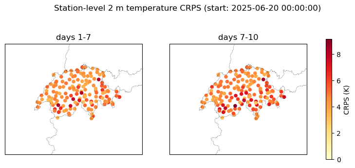
Station-level 2 m temperature CRPS maps averaged over medium/extended-range bins:

bins_dict = {
    "days 1-7": (np.timedelta64(24, "h"), np.timedelta64(7 * 24, "h")),
    "days 7-10": (np.timedelta64(7 * 24, "h"), np.timedelta64(10 * 24, "h")),
}

# plot args
# metric to plot
metric = "crps"
cmap = "YlOrRd"

# reduce all non-station dims: lead_time, valid_time (if present), member (if present)
plot_da = xr.concat(
    [
        metrics_ds["2m_temperature"]
        .sel(metric=metric, lead_time=slice(t0, t1))
        .mean(["lead_time", "valid_time", "member"])
        for t0, t1 in bins_dict.values()
    ],
    dim=pd.Index(list(bins_dict.keys()), name="bin"),
).rename(f"{metric.upper()} (K)")

proj = ccrs.LambertConformal(central_longitude=8)
extent = [*lon_slice, *lat_slice]
# vmax = float(plot_da.quantile(0.95))
norm = plt.Normalize(vmin=0, vmax=plot_da.max())

# plot
fig, axes = plt.subplots(1, 2, figsize=(10, 4), subplot_kw={"projection": proj})
for ax, bin_label in zip(axes, bins_dict):
    ax.scatter(
        plot_da.longitude.values,
        plot_da.latitude.values,
        c=plot_da.sel(bin=bin_label).values,
        cmap=cmap,
        norm=norm,
        s=20,
        transform=ccrs.PlateCarree(),
    )
    ax.coastlines(linewidth=0.6)
    ax.add_feature(cfeature.BORDERS, linestyle=":", linewidth=0.5)
    ax.set_extent(extent, crs=ccrs.PlateCarree())
    ax.set_title(bin_label)

fig.colorbar(
    plt.cm.ScalarMappable(norm=norm, cmap=cmap),
    ax=axes,
    label=f"{metric.upper()} (K)",
    shrink=0.8,
)
fig.suptitle(
    f"Station-level 2 m temperature {metric.upper()} "
    f"(start: {start_date.replace(tzinfo=None)})",
)

Text(0.5, 0.98, 'Station-level 2 m temperature CRPS (start: 2025-06-20 00:00:00)')

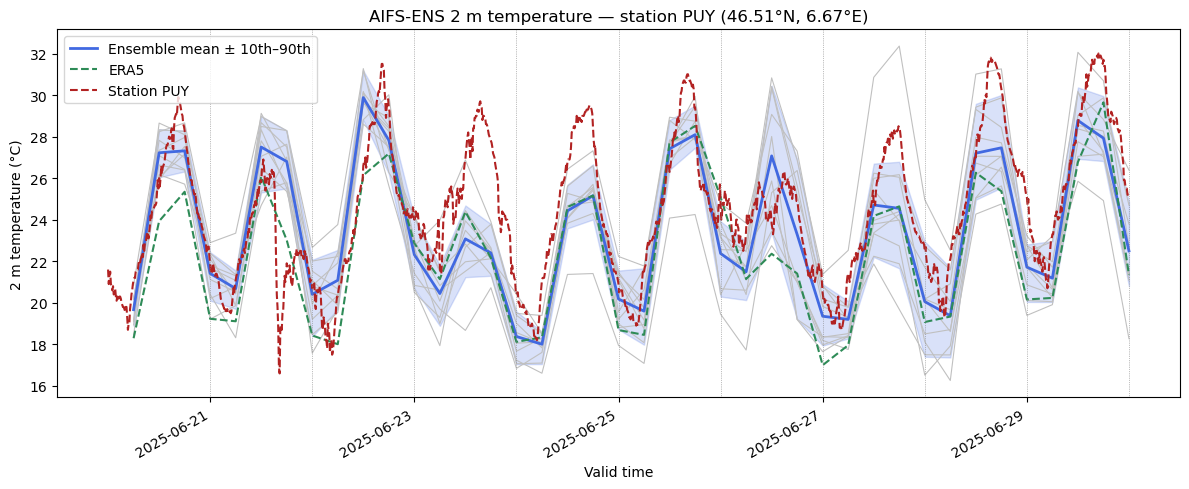
We conclude by plotting the 2 m temperature time series at a selected MeteoSwiss station, showing:

• AIFS individual members and ensemble mean with percentile envelope

• the selected station’s observations

• the ERA5 reference data

Note that this plot can take a while because forecast_ds["2t"] is chunked by ensembles.

station_id = "PUY"  # Pully, next to Lausanne

# station coordinates
stn_lat = float(ts_ds.latitude.sel(station_id=station_id))
stn_lon = float(ts_ds.longitude.sel(station_id=station_id))

# extract 2t at nearest grid point for all members, convert to °C
t2m_da = (
    forecast_ds["2t"].sel(lat=stn_lat, lon=stn_lon % 360, method="nearest") - 273.15
)

# ensemble long-form dataframe
# ACHTUNG: this is the expensive operation because it is where `compute` happens
ens_df = t2m_da.to_dataframe(name="2t").reset_index()

# station observations
obs_da = ts_ds["2m_temperature"].sel(station_id=station_id) - 273.15
obs_df = (
    obs_da.to_dataframe(name="2t").reset_index().rename(columns={"time": "valid_time"})
)

# get ERA5 reference
era5_ds = xr.open_dataset(era5_filepath)
era5_da = (
    era5_ds["2t"]
    .sel(latitude=stn_lat, longitude=stn_lon % 360, method="nearest")
    .isel(time=0)
    - 273.15
)
era5_valid_time = start_date + pd.to_timedelta(era5_da.prediction_timedelta.values)
era5_df = pd.DataFrame({"valid_time": era5_valid_time, "2t": era5_da.values})

# plot
fig, ax = plt.subplots(figsize=(12, 5))

# individual members (thin silver lines)
sns.lineplot(
    data=ens_df,
    x="valid_time",
    y="2t",
    units="ensemble_member",
    estimator=None,
    color="silver",
    linewidth=0.8,
    ax=ax,
)
# ensemble mean + 10th–90th CI (blue)
sns.lineplot(
    data=ens_df,
    x="valid_time",
    y="2t",
    estimator="mean",
    errorbar=("pi", 80),
    color="royalblue",
    linewidth=2,
    label="Ensemble mean ± 10th–90th",
    ax=ax,
)
# ERA5 (green dashed)
sns.lineplot(
    data=era5_df,
    x="valid_time",
    y="2t",
    color="seagreen",
    linewidth=1.5,
    linestyle="--",
    label="ERA5",
    ax=ax,
)
# station observations (red dashed)
sns.lineplot(
    data=obs_df,
    x="valid_time",
    y="2t",
    color="firebrick",
    linewidth=1.5,
    linestyle="--",
    label=f"Station {station_id}",
    ax=ax,
)

# final tweakings
# 24h vertical lines
for h in range(24, lead_time + 1, 24):
    ax.axvline(
        start_date + dt.timedelta(hours=h), color="grey", linestyle=":", linewidth=0.5
    )

# labels/titles
ax.set_ylabel("2 m temperature (°C)")
ax.set_xlabel("Valid time")
ax.set_title(
    f"AIFS-ENS 2 m temperature — station {station_id} "
    f"({stn_lat:.2f}°N, {stn_lon:.2f}°E)"
)
# legend
ax.legend()
# axis formatting for dates
fig.autofmt_xdate()
# tight layout
fig.tight_layout()