CMIP6-style SST patching: “what-if” scenario forecasts#
Because aifs-modal decouples ingestion from inference, any IC source that follows the Brightband zarr schema can be fed to the model. This notebook demonstrates that flexibility by constructing a modified set of initial conditions by (i) patching sea-surface temperatures (SSTs) with a CMIP6 end-of-century warming anomaly, (ii) writing them to a new ArrayLake repository, and (iii) running a forecast from it.
The recipe:
Run a baseline forecast from the Brightband IFS dataset on ArrayLake.
Compute a monthly SST anomaly from the Pangeo CMIP6 cloud archive (SSP5-8.5, 2050–2069 minus historical 1995–2014) and regrid it to the Brightband 0.25° lat/lon grid.
Open the Brightband source, apply the CMIP6 anomaly to skin temperature (
skt) and 2 m temperature (2t) over ocean (wherelsm < 0.5), and write the patched ICs to an ArrayLake repository.Run a forecast from the patched ICs and compare against the baseline.
Note
This notebook is primarily a library demo: it illustrates how to write custom ICs into an ArrayLake repository and run aifs-modal from them. The physical interpretation of a single-date, 4-day forecast response to a large SST anomaly is very limited.
import datetime as dt
import os

import arraylake
import gcsfs
import icechunk
import numpy as np
import pandas as pd
import scipy.interpolate
import xarray as xr

import plot_utils  # supplied alongside the other docs notebooks
from aifs_modal import app, run_forecast
_today_00z = dt.datetime.now(dt.UTC).replace(hour=0, minute=0, second=0, microsecond=0)
start_date = _today_00z - dt.timedelta(
    days=2
)  # safely within the Brightband ~15-day window
lead_time = 96  # hours

storage_bucket = "aifs-modal-unibe"
ifs_source_repo = "martibosch/ecmwf-ifs-hres-ics-open"  # Brightband ECMWF IFS dataset
patched_ics_repo = (
    "martibosch/aifs-modal-sst-2t-patched"  # ArrayLake repo for patched ICs
)
baseline_outputs_prefix = "aifs-outputs-ifs-baseline"
patched_outputs_prefix = "aifs-outputs-ifs-warm-2t-skt-patch"

# CMIP6 source for the SST anomaly (Pangeo cloud archive, anonymous GCS)
# Change source_id / institution to use a different model; check available
# combinations at https://pangeo-data.github.io/pangeo-cmip6-cloud/
cmip6_source_id = "IPSL-CM6A-LR"
cmip6_institution = "IPSL"
cmip6_member_id = "r1i1p1f1"
cmip6_hist_period = slice("1995", "2014")
cmip6_ssp_period = slice("2050", "2069")

print(f"start_date: {start_date.isoformat()}")
start_date: 2026-05-12T00:00:00+00:00
1. Run the baseline forecast#
with app.run():
    run_forecast.remote(
        start_date,
        storage_bucket,
        ic_source="ifs-arraylake",
        ic_source_repo=ifs_source_repo,
        lead_time=lead_time,
        outputs_prefix=baseline_outputs_prefix,
    )
2. Compute CMIP6 SST anomaly#
We load monthly mean sea-surface temperature (tos) from the Pangeo CMIP6 zarr archive on Google Cloud Storage and compute the SSP5-8.5 end-of-century anomaly relative to the historical baseline. The store URL is looked up from the Pangeo catalog CSV, which avoids hard-coding the gr vs gn grid-label that varies by model and variable. The anomaly is then regridded to the Brightband 0.25° lat/lon grid using scipy.interpolate.griddata, which handles both regular and curvilinear (e.g. IPSL ORCA1 tripolar) source grids.
Note
This step runs locally and requires gcsfs, pandas, and scipy (pip install gcsfs pandas scipy). Access is anonymous — no GCS credentials needed. The default model is IPSL-CM6A-LR; to use another, update cmip6_source_id, cmip6_institution, and cmip6_member_id in the setup cell.
fs = gcsfs.GCSFileSystem(token="anon", access="read_only")

print("Looking up CMIP6 catalog…")
catalog = pd.read_csv(
    "https://cmip6.storage.googleapis.com/pangeo-cmip6.csv",
    dtype=str,
)


def _cmip6_zstore(experiment_id, table_id="Omon", variable_id="tos"):
    activity = (  # noqa: F841
        "CMIP" if experiment_id == "historical" else "ScenarioMIP"
    )
    hits = catalog.query(
        "activity_id == @activity"
        " and institution_id == @cmip6_institution"
        " and source_id == @cmip6_source_id"
        " and experiment_id == @experiment_id"
        " and member_id == @cmip6_member_id"
        " and table_id == @table_id"
        " and variable_id == @variable_id"
    )
    if hits.empty:
        raise FileNotFoundError(
            f"No {variable_id}/{table_id} entry for {cmip6_source_id} {experiment_id} "
            "in Pangeo catalog. Browse https://pangeo-data.github.io/pangeo-cmip6-cloud/"
        )
    zstore = hits.sort_values("zstore").iloc[-1]["zstore"]
    print(f"  {experiment_id}: {zstore}")
    return zstore


print("Loading CMIP6 SST…")
tos_hist = (
    xr.open_zarr(
        fs.get_mapper(_cmip6_zstore("historical")), consolidated=True, chunks={}
    )["tos"]
    .sel(time=cmip6_hist_period)
    .groupby("time.month")
    .mean()
)
tos_ssp585 = (
    xr.open_zarr(fs.get_mapper(_cmip6_zstore("ssp585")), consolidated=True, chunks={})[
        "tos"
    ]
    .sel(time=cmip6_ssp_period)
    .groupby("time.month")
    .mean()
)
sst_anomaly = (tos_ssp585 - tos_hist).compute()  # (month=12, ...), NaN over land

# Regrid to regular 0.25° lat/lon grid — griddata handles both regular (1D) and
# curvilinear (2D, e.g. IPSL ORCA1 tripolar) source coordinate arrays.
target_lat = np.arange(90, -90.25, -0.25)  # (721,)
target_lon = np.arange(0, 360, 0.25)  # (1440,)
target_lon_g, target_lat_g = np.meshgrid(target_lon, target_lat)

month_field = sst_anomaly.sel(month=start_date.month)

# Resolve lat/lon coordinate arrays — try CF standard names first
lat_name = next(
    (c for c in ["latitude", "lat", "nav_lat"] if c in month_field.coords), None
)
lon_name = next(
    (c for c in ["longitude", "lon", "nav_lon"] if c in month_field.coords), None
)
src_lat = month_field.coords[lat_name].values  # (y,) or (y, x)
src_lon = month_field.coords[lon_name].values  # (x,) or (y, x)
if src_lat.ndim == 1:
    src_lon, src_lat = np.meshgrid(src_lon, src_lat)

src_vals = month_field.values.ravel()
src_lon_r = src_lon.ravel()
src_lat_r = src_lat.ravel()

# Normalize lon to [0, 360] so source and target share the same range
src_lon_r = np.where(src_lon_r < 0, src_lon_r + 360, src_lon_r)

valid = ~np.isnan(src_vals)
month_anomaly_025 = scipy.interpolate.griddata(
    np.column_stack([src_lon_r[valid], src_lat_r[valid]]),
    src_vals[valid],
    (target_lon_g, target_lat_g),
    method="linear",
    fill_value=0.0,
).astype("f4")  # (721, 1440); 0 where interpolation hull has no coverage

print(
    f"Month {start_date.month} SST anomaly "
    f"({cmip6_source_id} SSP5-8.5 {cmip6_ssp_period.start}–{cmip6_ssp_period.stop} "
    f"− hist {cmip6_hist_period.start}–{cmip6_hist_period.stop}): "
    f"mean={month_anomaly_025[month_anomaly_025 > 0].mean():.2f} K, "
    f"max={month_anomaly_025.max():.2f} K"
)
Looking up CMIP6 catalog…
Loading CMIP6 SST…
  historical: gs://cmip6/CMIP6/CMIP/IPSL/IPSL-CM6A-LR/historical/r1i1p1f1/Omon/tos/gn/v20180803/
  ssp585: gs://cmip6/CMIP6/ScenarioMIP/IPSL/IPSL-CM6A-LR/ssp585/r1i1p1f1/Omon/tos/gn/v20190903/
Month 5 SST anomaly (IPSL-CM6A-LR SSP5-8.5 2050–2069 − hist 1995–2014): mean=1.62 K, max=7.57 K
3. Write patched ICs to ArrayLake#
We read the two IC time steps needed by AIFS (start_date − 6 h and start_date) from the Brightband source, apply the CMIP6 anomaly to both skt (skin temperature, i.e. SST over ocean) and t2m (2 m air temperature), and write the result to an ArrayLake repository on main.
Patching both variables keeps the initial air–sea temperature gradient at its analysed value, so the model response reflects boundary warming rather than a day-0 surface-flux adjustment artefact.
Static fields (lsm, z_sfc, slor, sdor) are co-located on the same main branch so that ingest_ifs_arraylake can read them via ic_source_static_branch="main".
# client = arraylake.Client(token=os.environ["ARRAYLAKE_API_TOKEN"])
# alternatively, in this (local) notebook we can login interactively
client = arraylake.Client()
client.login()

# The two IC timestamps AIFS needs
init_times_np = np.array(
    [
        (start_date - dt.timedelta(hours=6)).replace(tzinfo=None),
        start_date.replace(tzinfo=None),
    ],
    dtype="datetime64[ns]",
)

patched_al = client.get_or_create_repo(patched_ics_repo)


def _ics_up_to_date(repo, init_times):
    """Return True if both IC timestamps are already committed on main."""
    try:
        session = repo.readonly_session("main")
        ds = xr.open_dataset(session.store, engine="zarr", zarr_format=3, chunks={})
        return bool(np.isin(init_times, ds.coords["init_time"].values).all())
    except Exception:
        return False


if _ics_up_to_date(patched_al, init_times_np):
    print(
        f"Patched ICs for {start_date.date()} already in {patched_ics_repo}, skipping."
    )
else:
    # Open Brightband source (dynamic on main, static on add-static-vars)
    source_al = client.get_repo(ifs_source_repo)
    dynamic_ds = xr.open_dataset(
        source_al.readonly_session("main").store,
        engine="zarr",
        zarr_format=3,
        chunks={},
    )
    static_ds = xr.open_dataset(
        source_al.readonly_session("add-static-vars").store,
        engine="zarr",
        zarr_format=3,
        chunks={},
    )

    patched = dynamic_ds.sel(init_time=init_times_np).isel(lead_time=[0]).compute()

    # Ocean mask from the Brightband static lsm (0.25° grid)
    lsm_arr = static_ds["lsm"].values
    while lsm_arr.ndim > 2:
        lsm_arr = lsm_arr.squeeze(axis=0)
    ocean = lsm_arr < 0.5  # (721, 1440)

    # Apply CMIP6 SST anomaly to skt and t2m at ocean points.
    # Note: Brightband stores 2m temperature as "t2m"; it is renamed to "2t" only
    # during IC ingestion into the Modal Volume.
    for varname in ("skt", "t2m"):
        arr = patched[varname].values.copy()
        arr[..., ocean] += month_anomaly_025[ocean]
        patched[varname] = xr.DataArray(
            arr, dims=patched[varname].dims, coords=patched[varname].coords
        )
    print(
        f"Patched skt+t2m: {ocean.sum()} ocean grid points, "
        f"mean anomaly = {month_anomaly_025[ocean].mean():.2f} K"
    )

    # Co-locate static fields (lsm, z_sfc, slor, sdor) on the same main branch so that
    # ingest_ifs_arraylake can read them with ic_source_static_branch="main"
    lat_dim, lon_dim = patched["skt"].dims[-2], patched["skt"].dims[-1]
    for varname in ["lsm", "z_sfc", "slor", "sdor"]:
        arr = static_ds[varname].values.astype("f4")
        while arr.ndim > 2:
            arr = arr.squeeze(axis=0)
        patched[varname] = xr.DataArray(arr, dims=[lat_dim, lon_dim])

    session = patched_al.writable_session("main")
    patched.to_zarr(session.store, zarr_format=3, mode="w")
    session.commit(
        f"CMIP6 {cmip6_source_id} SSP5-8.5 {cmip6_ssp_period.start}–"
        f"{cmip6_ssp_period.stop} SST anomaly applied to skt+t2m for "
        f"{start_date.date()}"
    )
    print(f"Patched ICs written to {patched_ics_repo} (main branch)")
4. Run the patched forecast#
Same run_forecast call as the baseline. ic_source_static_branch="main" tells ingest_ifs_arraylake to read both dynamic and static fields from main, where we wrote everything in step 3.
with app.run():
    run_forecast.remote(
        start_date,
        storage_bucket,
        ic_source="ifs-arraylake",
        ic_source_repo=patched_ics_repo,
        ic_source_static_branch="main",  # static fields co-located with dynamic on main
        lead_time=lead_time,
        outputs_prefix=patched_outputs_prefix,
    )
5. Compare baseline vs. patched#
Both forecasts are on the same 0.25° lat/lon grid, so we subtract them directly to isolate the 2 m temperature response to the warmer ocean boundary.
def open_forecast(prefix):
    storage = icechunk.tigris_storage(
        bucket=storage_bucket,
        prefix=prefix,
        region=os.getenv("AWS_REGION"),
        access_key_id=os.environ["AWS_ACCESS_KEY_ID"],
        secret_access_key=os.environ["AWS_SECRET_ACCESS_KEY"],
    )
    repo = icechunk.Repository.open(storage)
    session = repo.readonly_session("main")
    group = start_date.strftime("%Y-%m-%d/%Hz")
    return xr.open_dataset(
        session.store, group=group, engine="zarr", zarr_format=3, chunks={}
    )


ds_base = open_forecast(baseline_outputs_prefix)
ds_warm = open_forecast(patched_outputs_prefix)

# Compute only the 2t diff; then release the full datasets before plotting.
diff = (ds_warm["2t"] - ds_base["2t"]).isel(init_time=0).compute()
diff.name = "Δ 2 m temperature (skt+2t patch − baseline) [K]"
del ds_base, ds_warm
  2026-05-14T07:56:39.060680Z  WARN aws_runtime::env_config::normalize: profile [plugins] ignored; sections in the AWS config file (other than [default]) must have a prefix i.e. [profile my-profile]
    at /home/conda/feedstock_root/build_artifacts/icechunk_1776344638779/_build_env/.cargo/registry/src/index.crates.io-1949cf8c6b5b557f/aws-runtime-1.7.2/src/env_config/normalize.rs:121

  2026-05-14T07:56:40.728041Z  WARN aws_runtime::env_config::normalize: profile [plugins] ignored; sections in the AWS config file (other than [default]) must have a prefix i.e. [profile my-profile]
    at /home/conda/feedstock_root/build_artifacts/icechunk_1776344638779/_build_env/.cargo/registry/src/index.crates.io-1949cf8c6b5b557f/aws-runtime-1.7.2/src/env_config/normalize.rs:121
anomaly_label = (
    f"{cmip6_source_id} SSP5-8.5 {cmip6_ssp_period.start}–{cmip6_ssp_period.stop} "
    "anomaly"
)
g = plot_utils.make_cartopy_facet_plot(
    diff.isel(lead_time=slice(0, 8)),
    col="lead_time",
    cmap="RdBu_r",
    vmin=-3,
    vmax=3,
    cbar_kwargs={"shrink": 0.4, "pad": 0.02},
)
# ad-hoc tuning of vspace
# g.fig.subplots_adjust(hspace=0.05)
w, h = g.fig.get_size_inches()
g.fig.set_size_inches(w, h * 0.75)
g.set_titles("{value}")
g.fig.suptitle(f"Δ 2 m temperature — skt+2t patch ({anomaly_label})", y=1.02)
Text(0.5, 1.02, 'Δ 2 m temperature — skt+2t patch (IPSL-CM6A-LR SSP5-8.5 2050–2069 anomaly)')
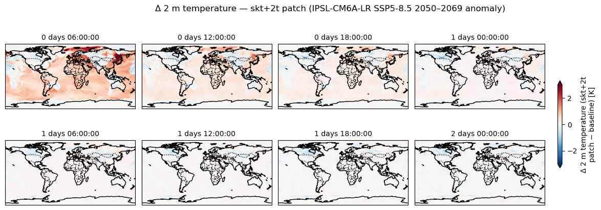
It seems like the anomaly that is clarly visible at +6h is practically gone after +24h, which is consistent with the limitations of current AI-based weather models in extrapolate and reliably forecast beyond their training domain (Zhang et al., 2026), but this is beyond the scope of this notebook.
Cleanup#
Remove all forecast data from the bucket:
import storage_utils

storage_utils.delete_prefixes(
    storage_bucket,
    baseline_outputs_prefix,
    patched_outputs_prefix,
)
deleted 3104 object(s) under s3://aifs-modal-unibe/aifs-outputs-ifs-baseline
deleted 2509 object(s) under s3://aifs-modal-unibe/aifs-outputs-ifs-warm-2t-skt-patch
done — removed 5613 objects from s3://aifs-modal-unibe/
References#
Zhongwei Zhang, Erich Fischer, Jakob Zscheischler, and Sebastian Engelke. Physics-based models outperform ai weather forecasts of record-breaking extremes. Science Advances, 12(18):eaec1433, 2026.